Download
1 / 29
300 likes | 498 Views
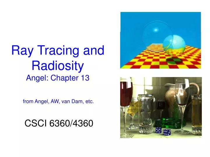
Ray Tracing and Radiosity Angel: Chapter 13 from Angel, AW, van Dam, etc. CSCI 6360/4360. Introduction. Recall, local vs. global illumination Local can’t consider interactions among elements, etc., shadows But, it is fast, and fast is good for interactive computer graphics. Introduction.

E N D
Ray Tracing andRadiosityAngel: Chapter 13 from Angel, AW, van Dam, etc. CSCI 6360/4360
Introduction • Recall, local vs. global illumination • Local can’t consider interactions among elements, etc., shadows • But, it is fast, and fast is good for interactive computer graphics
Introduction • Ray tracing is global • Can consider (essentially) all elements in scene/model world: • Shadows, reflections, mirrors, light transmission (translucent surfaces) • High visual realism – photorealism • Appel, 1968; Whitted, 1980 (recursive ray tracing)
Origins of Ray Tracing • Recall Durer’s painting showing perspective projection • Record string intersection from center of projection(eye) to the object as points on a 2D plane • Points created are perspective projection of 3D object onto 2D plane
About Ray Tracing • “Logical extension” to rendering with local lighting model • Note that most rays from light source do not pass through camera (or cop) • Do not contribute to image • Ray tracing • “Running illumination model backward” • An image precision approach • for each pixel – cast ray • Each ray either: • Strikes (intersects) object or light source • Goes off “to infinity” • Computing shade at point of intersection gives Phong (regular) shading!
About Ray Tracing • Computing shade at point of intersection gives Phong (regular) shading! • Only when consider further ray travel that difference emerge • Compute shadow, or feeler, rays from point on surface to each light source • If all surfaces are opaque and do not consider light scattered surface to surface, have image as before, but with shadows added
About Ray Tracing • For highly reflective surfaces best with ray tracing, can follow shadow ray until either goes off to infinity or intersects a light source • Recursive following is the norm • Particularly good at handling surfaces both reflective and transmissive • Some of light partially absorbed and contributes to diffuse reflection • Rest divided between reflected and transmitted ray • If light source visible at intersection point: • Compute contribution from light source, e.g., phong • Cast a ray in direction of perfect reflection • Cast a ray in direction of transmitted ray
About Ray Tracing • Figure shows single ray and path through an environment • Ray tree also shows tree • Note possibilities for parallelism • Rays can be traced independently from any point in tree • Will return with value • Theoretically, scattering at each point of intersection generates an infinite number of new rays that should be traced • In practice, only trace transmitted and reflected rays • Use Phong model to compute shade at point of intersection
Building a Ray Tracer • Best expressed recursively • Can remove recursion later • Image based approach • For each ray ……. : • Find intersection with closest surface • Need whole object database available • Complexity of calculation limits object types • Compute lighting at surface • Trace reflected and transmitted rays • Determining intersections … is a more involved topic
When to Stop • Some light will be absorbed at each intersection • Track amount left • Ignore rays that go off to infinity • Put large sphere around problem • Just another object • 2D case at right • Count steps • Put a limit (vs. infinity) on number of step that are traced
Recursive Ray Tracer - Angel // Returns illumination value (color) for subtrees // (which contributes to final), and finally for pixel color c = trace(point p, vector d, int step) { color local, reflected, transmitted; point q; normal n; enum status; if(step > max) return(background_color); q = intersect(p, d, status); if(status==light_source) return(light_source_color); if(status==no_intersection) return(background_color); n = normal(q); r = reflect(q, n); t = transmit(q,n); local = phong(q, n, r); reflected = trace(q, r, step+1); transmitted = trace(q, t, step+1); return(local+reflected+transmitted); }
Recursive Ray Tracer – Var Names // Returns illumination value (color) for subtrees // (which contributes to final), and finally for pixel color c = trace(point start-pt, vector start-dir, int step) { if(step > max) return(background_color); intersect-pt = intersect(start-pt, start-dir, status); if(status==light_source) return(light_source_color); if(status==no_intersection) return(background_color); n = normal(intersect-pt); intersect-pt = reflect(intersect-pt, n); transmit-direction = transmit(intersect-pt, n); local = phong(intersect-pt, n, intersect-pt); reflected = trace(intersect-pt, reflected-direction, step+1); transmitted = trace(intersect-pt, transmit-direction, step+1); return(local + reflected + transmitted); }
Real-time Ray Tracing (van Dam 2010) • Traditionally computationally impossible to do in real-time • Hard to make hardware optimized for ray tracing: • Large amount of floating point calculations • Complex control flow structure • Complex memory access for scene data • One solution: software-based, highly optimized raytracer using cluster with multiple CPUs • Hard to have widespread adoption because of size and cost • May be possible with the advance of commercially available multi-core CPUs • E.g., PC CPUs up to 16 cores • Example: OpenRT project http://openrt.de OpenRT rendering of five maple trees And 28,000 sunflowers (35,000 triangles) on 48 CPUs
Real-time Ray Tracing(van Dam 2010) • Another solution: Use regular GPU’s to speed up ray tracing • Difficult: GPU traditionally specialized for rasterization • NVIDIA at SIGGRAPH 2010: demos HD resolution ray tracing at 30fps • Uses four GPUs in parallel, running NVIDIA CUDA architecture (codename Fermi): http://www.nvidia.com/object/fermi_architecture.html • Next-generation NVIDIA GPUs contain 512 cores each, total of 2048 cores! • Interactive ray tracing demo: • http://www.nvidia.com/object/quadro-fermi-video-view09.html • Three times increase in rendering performance since SIGGRAPH 2008 • Currently fastest solution to real-time ray tracing
Real-time Ray Tracing(van Dam 2010) • Yet another solution: custom hardware for doing ray tracing • Custom chip with sole purpose of performing ray tracing • Example: RPU, a custom chip to do ray tracing proposed at SIGGRAPH 2005. • http://graphics.cs.uni-b.de/~woop/rpu/rpu.html • 66 MHz prototype outperforms OpenRT running on a 2.66 GHz Intel Pentium 4 A scene (52,470 triangles) taken from the game UT2003 rendered in RPU
POV-Ray • Public domain ray tracer • povray.org • “The Persistence of Vision Raytracer is a high-quality, totally free tool for creating stunning three-dimensional graphics. It is available in official versions for Windows, Mac OS/Mac OS X and i86 Linux. The source code is available for those wanting to do their own ports.”
End • .
Introduction • Radiosity is another global illumination technique • Local can’t consider interactions among elements, etc., shadows • But, it is fast, and fast is good for interactive computer graphics • Ray tracing works well with reflective surface, but not diffuse • Radiosity works especially well for diffuse-diffuse interactions not captured by other models • At right light reflected from walls will be considered • For other models reflected light color not change • Recall BRDF – and general rendering equation • Radiosity uses/solves special case of diffuse-diffuse interactions to greatly simplify it application
Physical Model: BRDF Bidirectional Reflectance Distribution Function • Light energy can arrive at any point on a surface from any direction and be reflected and leave from any direction • For every pair of input and output directions, will be a value that is the fraction of incoming light that is reflected and leave in output direction • BDRF – Bidirectional reflectance distribution function • Describes reflectance, absorption, and transmission of light at surface of material • BDRF is a function of • Frequency of light • 2 angles to describe light in • 2 angles to describe light out
Introduction • Basic idea is to break scene into small, flat polygons (patches) • Each assumed to be perfectly diffuse and renders in a single shade • Finding shades provides color to 3D environment • Then, can just place viewer in environment and render with a pipeline architecture • “The radiosity equation” …
Terminology • Energy ~ light (incident, transmitted) • Must be conserved • Energy flux = luminous flux = power = energy/unit time • Measured in lumens • Depends on wavelength so we can integrate over spectrum using luminous efficiency curve of sensor • Energy density (Φ) = energy flux/unit area • Intensity <> brightness • Brightness is perceptual = flux/area-solid angle = power/unit projected area per solid angle • Measured in candela Φ = ∫ ∫ I dA dω
Rendering Equation • Outgoing light is from two sources • Emission • Reflection of incoming light • Must integrate over all incoming light • Integrate over hemisphere • Would be very computationally expense • As noted, radiosity uses patches N Iin(Φin) Iout(Φout)
Rendering Equation • Rendering equation is an energy balance • Energy in = energy out • Integrate over hemisphere • Fredholm integral equation • Cannot be solved analytically in general • Various approximations of Rbd give standard rendering models • Should also add an occlusion term in front of right side to account for other objects blocking light from reaching surface N Iin(Φin) Iout(Φout)
Radiosity Equation • Again, • Consider objects to be broken up into flat patches (which may correspond to the polygons in the model) • Assume that patches are perfectly diffuse reflectors • Radiosity = flux = energy/unit area/ unit time leaving patch • Energy balance, form factor, sum of energy from each i patch • biai = eiai + ρi ∑ fjibjaj • Form factor between patch i and j, fraction of light leaving patch I that reaches j • Given, reciprocity (below), substitute in above to give radiosity eq. • fijai = fjiaj • Radiosity equation • bi = ei + ρi ∑ fijbj
Solution • Angel details practical matrix form solution
Practical Considerations • Have considered hemisphere of patches • Use illuminating hemisphere • Center hemisphere on patch with normal pointing up • Must shift hemisphere for each point on patch • Easier to use a hemicube instead of a hemisphere in practice • Rule each side into “pixels” • Easier to project on pixels which give delta form factors that can be added up to give desired from factor • To get a delta form factor we need only cast a ray through each pixel
And … “Instant Radiosity” • Want to use graphics system, if possible • Suppose we make patch emissive (recall from OpenGL) • The light from this patch is distributed among other patches • Shade of other patches approximately form factors! • Must use multiple OpenGL point sources to approximate a uniformly emissive patch • And can thus perform radiosity calculations with standard pipeline architecture!
End • .