Download
1 / 60
600 likes | 717 Views
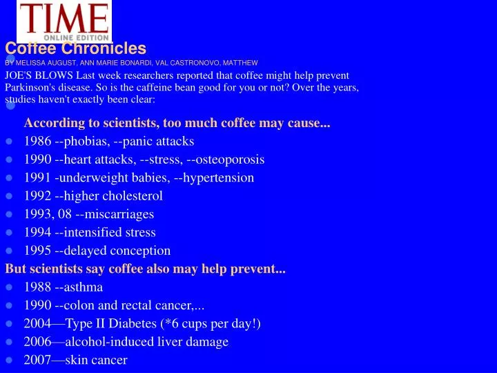
Coffee Chronicles BY MELISSA AUGUST, ANN MARIE BONARDI, VAL CASTRONOVO, MATTHEW JOE'S BLOWS Last week researchers reported that coffee might help prevent Parkinson's disease. So is the caffeine bean good for you or not? Over the years, studies haven't exactly been clear:.

E N D
Coffee Chronicles BYMELISSA AUGUST, ANN MARIE BONARDI, VAL CASTRONOVO, MATTHEW JOE'S BLOWS Last week researchers reported that coffee might help prevent Parkinson's disease. So is the caffeine bean good for you or not? Over the years, studies haven't exactly been clear: • According to scientists, too much coffee may cause... • 1986 --phobias, --panic attacks • 1990 --heart attacks, --stress, --osteoporosis • 1991 -underweight babies, --hypertension • 1992 --higher cholesterol • 1993, 08 --miscarriages • 1994 --intensified stress • 1995 --delayed conception But scientists say coffee also may help prevent... • 1988 --asthma • 1990 --colon and rectal cancer,... • 2004—Type II Diabetes (*6 cups per day!) • 2006—alcohol-induced liver damage • 2007—skin cancer
? Exposure Disease Medical Studies The General Idea… Evaluate whether a risk factor (or preventative factor) increases (or decreases) your risk for an outcome (usually disease, death or intermediary to disease).
Exposure (E) No Exposure (~E) Disease (D) a b (a+b)/T = P(D) No Disease (~D) c d (c+d)/T = P(~D) (a+c)/T = P(E) (b+d)/T = P(~E) Marginal probability of exposure Marginal probability of disease General 2x2 Table N
Risk Ratio ( Relative Risk) Risk ratio is used to compare the risk for two groups An risk of 1 means there is no difference between the groups.
Coronary calcificationis a process in which the interior lining of the coronary arteries develops a layer of hard substance known as plaque. Excessive amounts of cholesterol, fat, and waste material become calcified in arteries that have been weakened or damaged due to smoking, high blood pressure, diabetes, or a generally unhealthy diet. Coronary calcification restricts blood flow, presenting the risk of chronic chest pain, heart attacks, and eventual heart failure.Is depression and coronary calcification is associated
Any depression None 28 511 53 1328 Coronary calc >500 539 1381 Coronary calc <=500 81 1839 1920 Difference of proportions Z-test:
Or, use relative risk (risk ratio) Compare the risk for each groups Any depression None 28 511 53 1328 Coronary calc >500 539 1381 Coronary calc <=500 81 1839 1920 See how to get this in R Interpretation: those with coronary calcification are 35% more likely to have depression (not significant).
Any depression Any depression None None 539*81/1920= 22.7 28 539-22.7= 516.3 511 81-22.7= 58.3 53 1328 1381-58.3= 1322.7 Coronary calc >500 Coronary calc >500 539 539 1381 1381 Coronary calc <=500 Coronary calc <=500 81 81 1839 1839 1920 1920 Or, use chi-square test: Observed: Expected:
Chi-square test: Note: 1.77 = 1.332
Chi-square test also works for bigger contingency tables (RxC):
Chi-square test also works for bigger contingency tables (RxC):
Observed: Expected:
? Biological changes Lack of exercise Poor Eating ? Cause and effect? depression in elderly atherosclerosis
? Biological changes Lack of exercise Poor Eating ? Advancing Age Confounding? depression in elderly atherosclerosis
Cross-Sectional Studies • Advantages: • cheap and easy • generalizable • good for characteristics that (generally) don’t change like genes or gender • Disadvantages • difficult to determine cause and effect • problematic for rare diseases and exposures
2. Cohort studies: Sample on exposure status and track disease development (for rare exposures) • Marginal probabilities (and rates) of developing disease for exposure groups are valid.
Example: The Framingham Heart Study • The Framingham Heart Study was established in 1948, when 5209 residents of Framingham, Mass, aged 28 to 62 years, were enrolled in a prospective epidemiologic cohort study. • Health and lifestyle factors were measured (blood pressure, weight, exercise, etc.). • Interim cardiovascular events were ascertained from medical histories, physical examinations, ECGs, and review of interim medical record.
Example 2: Johns Hopkins Precursors Study(medical students 1948 through 1964) http://www.jhu.edu/~jhumag/0601web/study.html From the John Hopkin’s Magazine website (URL above).
Exposed Disease-free cohort Not Exposed Cohort Studies Disease Disease-free Target population Disease Disease-free TIME
Exposure (E) No Exposure (~E) Disease (D) a b No Disease (~D) c d a+c b+d risk to the exposed risk to the unexposed The Risk Ratio, or Relative Risk (RR)
Normal BP Congestive Heart Failure High Systolic BP No CHF 400 400 1500 3000 1100 2600 Hypothetical Data
Case-Control Studies Sample on disease status and ask retrospectively about exposures (for rare diseases) • Marginal probabilities of exposure for cases and controls are valid. • Doesn’t require knowledge of the absolute risks of disease • For rare diseases, can approximate relative risk
Case-Control Studies Disease (Cases) Exposed in past Not exposed Target population Exposed No Disease (Controls) Not Exposed
Example: the AIDS epidemic in the early 1980’s • Early, case-control studies among AIDS cases and matched controls indicated that AIDS was transmitted by sexual contact or blood products. • In 1982, an early case-control study matched AIDS cases to controls and found a positive association between amyl nitrites (“poppers”) and AIDS; odds ratio of 8.6 (Marmor et al. 1982). This is an example of confounding.
Case-Control Studies Examples • Case-control studies identified associations between lip cancer and pipe smoking (Broders 1920), breast cancer and reproductive history (Lane-Claypon 1926) and between oral cancer and pipe smoking (Lombard and Doering 1928). All rare diseases. • Case-control studies identified an association between smoking and lung cancer in the 1950’s.
Case-control example • A study of the relation between body mass index and the incidence of age-related macular degeneration (Moeini et al. Br. J. Ophthalmol, 2005). • Methods: Researchers compared 50 Iranian patients with confirmed age-related macular degeneration and 80 control subjects with respect to BMI, smoking habits, hypertension, and diabetes. The researchers were specifically interested in the relationship of BMI to age-related macular degeneration.
Overweight Normal ARMD 27 23 No ARMD 54 26 Corresponding 2x2 Table 50 80 What is the risk ratio here? Tricky: There is no risk ratio, because we cannot calculate the risk of disease!!
The odds ratio… • We cannot calculate a risk ratio from a case-control study. • BUT, we can calculate a measure called the odds ratio…
Odds vs. Risk 1:1 3:1 1:9 1:99 Note: An odds is always higher than its corresponding probability, unless the probability is 100%.
Exposure (E) No Exposure (~E) Disease (D) a b No Disease (~D) c d Odds of exposure in the cases The proportion of cases and controls are set by the investigator; therefore, they do not represent the risk (probability) of developing disease. Odds of exposure in the controls The Odds Ratio (OR) a+b=cases c+d=controls
Exposure (E) No Exposure (~E) Disease (D) a b No Disease (~D) c d Odds of exposure for the cases. Odds of disease for the exposed Odds of diseasefor the unexposed Odds of exposure for the controls The Odds Ratio (OR)
Odds of exposure in the cases Odds of exposure in the controls Bayes’ Rule Odds of disease in the exposed What we want! Odds of disease in the unexposed Proof via Bayes’ Rule (optional) =
Overweight Normal ARMD a b No ARMD c d Odds of overweight for the cases. Odds of ARMD for the overweight Odds of ARMD for the normal weight Odds of overweight for the controls The Odds Ratio (OR)
Overweight Normal ARMD 27 23 No ARMD 54 26 The Odds Ratio (OR)
Overweight Normal ARMD 27 23 No ARMD 54 26 The Odds Ratio (OR) Can be interpreted as: Overweight people have a 43% decrease in their ODDS of age-related macular degeneration. (not statistically significant here)
The odds ratio is a good approximation of the risk ratio if the disease is rare. If the disease is rare (affecting <10% of the population), then: WHY? If the disease is rare, the probability of it NOT happening is close to 1, and the odds is close to the risk. Eg:
Who is Fisher Ronald Aylmer Fisher (17 February 1890 – 29 July 1962) was an Englishstatistician, evolutionary biologist, geneticist, and eugenicist. Fisher is known as one of the chief architects of the neo-Darwinian synthesis, for his important contributions to statistics, including the analysis of variance (ANOVA), method of maximum likelihood, fiducial inference, and the derivation of various sampling distributions, and for being one of the three principal founders of population genetics. Anders Hald called him "a genius who almost single-handedly created the foundations for modern statistical science", while Richard Dawkins named him "the greatest biologist since Darwin".
Fisher’s “Tea-tasting experiment” Claim: Fisher’s colleague (call Dr. Muriel Bristol”) claimed that, when drinking tea, she could distinguish whether milk or tea was added to the cup first. To test her claim, Fisher designed an experiment in which she tasted 8 cups of tea (4 cups had milk poured first, 4 had tea poured first). Null hypothesis: Cathy’s guessing abilities are no better than chance. Alternatives hypotheses: Right-tail: She guesses right more than expected by chance. Left-tail: She guesses wrong more than expected by chance
Milk Tea Milk 3 1 Tea 1 3 Guess poured first Poured First 4 4 Fisher’s “Tea-tasting experiment” Experimental Results:
Milk Milk Tea Tea Milk Milk 3 4 1 0 Tea Tea 0 1 4 3 Guess poured first Guess poured first Poured First Poured First 4 4 4 4 Fisher’s Exact Test Step 1: Identify tables that are as extreme or more extreme than what actually happened: Here she identified 3 out of 4 of the milk-poured-first teas correctly. Is that good luck or real talent? The only way she could have done better is if she identified 4 of 4 correct.
Milk Milk Tea Tea Milk Milk 3 4 1 0 Tea Tea 0 1 4 3 Guess poured first Guess poured first Poured First Poured First 4 4 4 4 Fisher’s Exact Test Step 2: Calculate the probability of the tables (assuming fixed marginals)
Step 3: to get the left tail and right-tail p-values, consider the probability mass function: Probability mass function of X, where X= the number of correct identifications of the cups with milk-poured-first: “right-hand tail probability”: p=.243 “left-hand tail probability” (testing the alternative hypothesis that she’s systematically wrong): p=.986 R also gives a “two-sided p-value” which is calculated by adding up all probabilities in the distribution that are less than or equal to the probability of the observed table (“equal or more extreme”). Here: 0.229+.014+.0.229+.014= .4857 See R code in file 2by2table.R on my website
1 1 When a disease is rare: P(~D) = 1 - P(D) 1 The rare disease assumption
Odds ratio Odds ratio Odds ratio Risk ratio Risk ratio Odds ratio Risk ratio Risk ratio The odds ratio vs. the risk ratio Rare Outcome 1.0 (null) Common Outcome 1.0 (null)
General Rule of Thumb: “OR is a good approximation as long as the probability of the outcome in the unexposed is less than 10%” Prevalence of age-related macular degeneration is about 6.5% in people over 40 in the US (according to a 2011 estimate). So, the OR is a reasonable approximation of the RR. When is the OR is a good approximation of the RR?