Download
1 / 20
200 likes | 369 Views
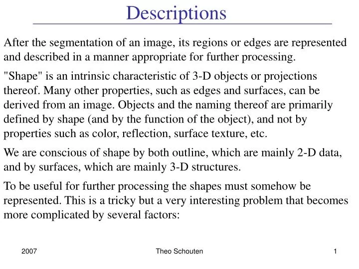
Descriptions. After the segmentation of an image, its regions or edges are represented and described in a manner appropriate for further processing.

E N D
Descriptions After the segmentation of an image, its regions or edges are represented and described in a manner appropriate for further processing. "Shape" is an intrinsic characteristic of 3-D objects or projections thereof. Many other properties, such as edges and surfaces, can be derived from an image. Objects and the naming thereof are primarily defined by shape (and by the function of the object), and not by properties such as color, reflection, surface texture, etc. We are conscious of shape by both outline, which are mainly 2-D data, and by surfaces, which are mainly 3-D structures. To be useful for further processing the shapes must somehow be represented. This is a tricky but a very interesting problem that becomes more complicated by several factors: Theo Schouten
problems -Shapes are often complex. Color, motion and intensity can be quantified by a small number of well-understood parameters. Shape can often only be explicitly represented using hundreds of parameters. It is not clear which aspects or features of shape are important for recognition and which can decrease the complexity. -Introspection does not help. A large amount of the human brains seems to work on shape recognition. However, this activity occurs primarily subconsciously. Why is shape recognition (think of faces for example) so easy for a human and shape description so difficult? We do not have a precise language for shapes (we speak of egg-shaped or ellipse-shaped). - There is little mathematical guidance. Math has traditionally not used "computational geometry". For example, just recently a mathematical definition of a “solid object" has been given which coincides with our intuition of set operations on solid objects. - This field of expertise is young, only recently it is useful to represent complex shapes in a manner that a computer can read, edit and graphically represent them. There are no generally accepted representation schemas for all types of shapes; there are several with each their own advantages and disadvantages for certain applications. Algorithms for the manipulation of shapes (for example, how to carry a couch up the stairs) are extremely complex, and still in a rudimentary stage. Theo Schouten
Chain codes, signatures Theo Schouten
Polygonal approximations An edge can each be approximated to any desired precision by a polyline. Finding a polyline approximation for a certain edge is a segmentation problem: finding the corner points or breakpoints that yield a good or a best polyline approximation (according to a certain criterion). Just as with regional segmentation, methods can also be characterized by the concepts "merging" and "splitting". This tolerance band method usually does not find the most economical set of segments. This is a general problem of these "one-pass" algorithms, a new break point is only taken when something went wrong, but it is often desired to take a new break point at an earlier stage. Afterwards one can try to find a better solution by shifting certain break points. Split method Theo Schouten
Spatial Occupation-Matrix The y-axis representation is a run-length coding in the y-direction of the spatial occupation-matrix. There are several possibilities to do this:{ (2,2,3), (4,4,4,6,6), (5,4,6), (6,6,6)} (starty, startx, stopx){ (8), (1,2,5), (8), (3,1,1,1,2), (3,3,2), (5,1,2), (8), (8)}: for each y the length of 0,1,0,... rows Union and intersection can be implemented as sorting and joining operations on the RLE rows, with a timescale initially proportional to the number of y rows. This representation is more compact than the occupation-matrix, except when there are long structures in the y-direction. Quad trees are another manner of coding the spatial occupation-matrix. The image is recursively divided into four parts until every region is composed solely out of a 1 or 0. They can easily be constructed from an intermediate pyramid structure and stored as a linear structure. Theo Schouten
Skeleton of a region The medial-axis of an area A is a set of pairs:{x,ds(x,B)} with ds(x,B) = min {d(x,z), z in B: the boundary of the region}such that the union of the circles with center x and radius ds(x,B) is equal to that of region A. This skeleton is very sensitive to noise on the boundary, which can be prevented by smoothing the edge. Distance transformations Medial-axis is set of local maxima Original image 4-neighbor DT 8-neighbor DT Theo Schouten
DT’s • Many DT algorithms for different distance measures are possible: • 4 neighbor: the minimum number of steps required to reach a 0 via 4-neighbors- 8 neighbor: via 8 neighbors, always smaller or equal to the 4-neighbor distance- approximations of euclidian (chamfer distances Borgefors, 1986 ) • Euclidian: the real Euclidian distance • There are parallel and serial versions. Thinning algorithms, of which there are many, shrink a (binary) region until there is a sort of median left over, which is then used for further processing and editing. The distance information is not stored, therefore the original image cannot be reconstructed. Theo Schouten
Shape numbers Shape numbers of order n, related to their chain code of length n, can be given to edges. The derivative of the chain code with length n is rotated such that the smallest value is attained. This shape number is independent of the position and orientation of the object. It is also independent of the scaling of the object, only dependent on the relative proportions between scale and size of the digitization grid. By changing the size of this grid, "shape numbers" of different orders can be attained. The lower the order, the coarser the digitalization, and the smaller the differences between the shapes become. Theo Schouten
Comparing shapes The highest order, at which two shapes still have the same shape number, is an indication of equality of the shapes . Theo Schouten
Fourier descriptors The curve (s)= (s) - 2 s/P is used as a basis for the shape description by Fourier transformation. Some shape parameters are determined by using the amplitudes of the lower order Fourier components. These parameters give an indication of the "pointiness" of the shape. A Fourier description can also be determined directly from the shape, using (x,y) as a complex number x+jy. A shape is usually well described by a small amount of lower order Xk terms. These are not invariant under rotation, translation and scaling, but combinations can be determined that do have those properties. Theo Schouten
Region characteristics The are several measures for the eccentricity. For example, if A is a piece of string of the maximum length, B the string perpendicular to A and also of maximal length, then: = A / B A unit for the compactness is the ratio: circumference2 / surface area. This is minimal for a circle (4). This can easily be calculated from the chain-code. This method is not appropriate for smaller discrete objects. Other eccentricity units are based on moments: Mij = R (x0-x)i(y0-y)j with x0 = (1/n) R x and y0 = (1/n) R y The orientation of a region (the angle between the main axis of the region to the x-axis) and are given by: tan 2 = 2 M11 / ( M20 - M02 ) = ( ( M20 - M02 ) 2 + 4 M11) / surface area Theo Schouten
Moments Moments for a gray image:µpq = xy (x-x0)p (y-y0)q f[x,y] A uniqueness theorem states that if f(x,y) is continuous and only unequal to 0 in a restricted area, then the series µpq is uniquely determined by f(x,y) and vice versa. From the second and third order moments a set of seven invariant moments can be calculated, which do not change during translation, scaling and rotation of a region.In practice it is very difficult to use these moments for the recognition of objects. Theo Schouten
Textures A possible description of texture is: "an image is built up of many interweaved elements". The idea of interweaved elements is closely related to the idea of texture resolution, something like the average number of pixels needed to describe each texture element. If this is large enough, one can try to describe the individual elements with some detail and especially their positions. When this number comes close to 1, it is more difficult to characterize individual elements. Statistical methods are then used to describe the distribution of the gray levels in the image. Theo Schouten
hierarchical, gradient Textures can be hierarchical, different levels correspond to different recording resolutions. When we look at a brick wall closely, we see that each brick has color or intensity variations which we can describe using a statistical model. If we look at the wall at a larger distance, then we can recognize half or whole bricks and describe the location and orientation of those bricks relative to each other. At an even larger distance each individual brick will only be several pixels large and is not suitable for geometric descriptions, we must then migrate to a more suitable statistical model. Texture is almost always a characteristic bound to a region. It can therefore be used to determine the properties of the region, such as the orientation with respect to the viewing direction, or the distance, to the camera: the so called texture gradient techniques. Theo Schouten
Statistical pattern recognition Statistical pattern recognition occupies itself with the classification of (individual occurrences) patterns. It is a separate field of expertise and has many application possibilities. A basic notation in pattern recognition is the "feature vector", v = (v1,...,vn), with which the relevant properties of a pattern are represented in a small n-dimensional Euclidian space. The feature vector is calculated out of available measurement data. With effective features the different classes can be divided into well-defined sub-spaces. The vectors of instances of a certain class lie close to each other and are well separated from vectors in other classes. • Suitable features and a good partition of the feature space can be achieved by: • analytical methods: when parametric models of textures are available. • training: use several texture instances of each class. Think up features and vary these to minimize distances within the classes and to maximize the inter-class distances. • learning: take several textures, calculate possible feature spaces and in that try to find spatial clusters. Try to identify the texture classes using those clusters. Theo Schouten
Classification methods The "nearest mean" or "minimum distance" method. Every texture class i has a center point ci in the n-dimensional feature space. It is determined by training, for example by averaging the training samples of each class. A new point, for which the Euclidian distance || v - ci||2 is minimal, to class i. - "nearest neighbour" classifier: take the training sample which lie closest to the new point, take that class as the class of the new point. - With the "condensed nearest neighbor" classification we are only interested in the training samples that lie on the edge of each class subspace. - With the "k-Nearest Neighbour" (kNN) classifier we are interested in the k training samples that are the closest to the new point. We take the most occuring class. Theo Schouten
Fourier features Vr1,r2 = |F(u,v)|2 dudv r12 (u2 + v2) < r22 V 1, 2=|F(u,v)|2 dudvwith over 1 tan-1(v/u) < 2 Theo Schouten
Laws method • We can also apply a similar sort of energy approximation to the spatial image itself. The advantage is that the basis is not the Fourier basis (cos and sin waves) but rather a more suitable set of basic texture patterns. An example of Laws (1980): • first flatten the gray level histogram by transforming the gray levels, this eliminates the influence of the lighting. • decompose the image (as with Frei-Chen) into m 5*5 or 3*3 basic texture patterns. This results in m images: f'k = f hk • determine the "energy" by averaging with the 15 * 15 surrounding environment (texture is a regional characteristic): f"k (x,y) = (1/225) | f'k (x',y')| with |x-x'| < 7 and |y-y'| <7 • this f"k defines a m-dimensional feature vector for each pixel (x,y):v(x,y) = { f"1 (x,y), f"2 (x,y),..., f"m (x,y) } Theo Schouten
Construction kernels An alternative, that which Laws used, is to construct about 25 5*5 convolution kernels from 5 one-dimensional kernels. This is done by the convolution of one horizontal 1-D kernel with one vertical 1-D kernel: L5 = [ 1 4 6 4 1 ] (Level)E5 = [ -1 -2 0 2 1 ] (Edge)S5 = [ -1 0 2 0 -1 ] (Spot)W5 = [ -1 2 0 -2 1 ] (Wave)R5 = [ 1 -4 6 -4 1 ] (Ripple) If the direction of the texture is not of importance, the features can be averaged to a set of 14 features that remain invariant under the rotation of the texture. Theo Schouten
SGLD Spatial Gray Level Dependence (SGLD) matrices (sometimes also referred to as co-occurrence matrices) are one of the most popular sources of texture features. The definition of the SGLD matrix is: S(i,j,d, ) : the number of locations (x,y) in the image f with f(x,y) = i and f(x + d cos , y + d sin ) = j; i and j are gray values, usually in bins: minI, minI+ I,...., maxI d the distance, smaller than the texel size (a small number of pixels) usually restricts itself to a small number of angles (steps of 45°) For many textures the reversal of the direction is not relevant: S'(d, ) = 1/2 ( S(d, ) + S(d, + ) ) Some features which can be derived from the SGLD matrix are: E(d, ) = i j S(i,j,d, )2 (Energy) H(d, ) = i j S(i,j,d, ) ln S(i,j,d, ) (Entropy) I(d, ) = i j (i-j)2 S(i,j,d, ) (Inertia, contrast) These features have no relationship with "rough" or "smooth" which people typically use to describe textures. Theo Schouten