Download

1 / 60
610 likes | 618 Views
World Dynamics. In this lecture, we shall apply the system dynamics modeling methodology to the problem of making predictions about the future of our planet.

E N D
World Dynamics In this lecture, we shall apply the system dynamics modelingmethodology to the problem of making predictions about the future of our planet. This has been one of the most spectacular --and also most controversial-- of all applications of this methodology reported to this day.
Forrester’s world model (World2) 1st modification: reduce utilization of natural resources 2nd modification: reduce pollution 3rd modification: reduce death rate 4th modification: simulate backward through time 5th modification: optimize resource utilization Meadows’ world model (World3) Table of Contents
In 1971, J.W. Forrester published a model, that he had developed for the Club of Rome, offering predictions about the future of our planet. The model makes use of his system dynamics modeling methodology. It is an extremely simple 5th-order differential equation model. He sold immediately several million copies of his book, which was also quickly translated into many languages. He was strongly criticized for his model by many of his colleagues. Forrester’s World Model
Which variables should be used as state variables? How many of those are needed? There obviously is no good answer to these questions. It takes either genius or recklessness to even come up with a meaningful answer. Forrester decided that world population is a natural candidate to be chosen as an important state variable, as the world approaches its limits to growth. Another important variable is pollution, as too much pollution will clearly have tremendous effects on the ecological balance of the globe. Selection of State Variables I
A third good candidate is the amount of irrecoverable natural resources left. In 1971, it may have required vision to recognize that the exhaustion of fossil fuels will affect us in dramatic ways. Today, this is evident to us all. A fourth candidate is world capital investment. More investment means more wealth, but also more pollution. A fifth and final candidate is the percentage of capital invested in the agricultural sector. We evidently need food, and available capital can be invested in growing food. Selection of State Variables II
Each state variable was given a single inflow and a single outflow rate, except for the natural resources, which are only depleted. Let us look at the laundry list for the birth rate. Forrester postulated that the birth rate depends on: It may make sense to postulate that the birth rate grows proportionally with the population, thus: Birth_rate = f (Population, Pollution, Food, Crowding, Material_Standard_of_Living) Birth_rate = Population · f (Pollution, Food, Crowding, Material_Standard_of_Living) Rate Variables and Laundry Lists I
Since functions of four variables are difficult to identify, and at least, call for many observations, Forrester proposed a simplifying assumption: each multi-valued function can be represented as a product of single-valued functions: This assumption certainly is daring, but so is the entire enterprise. Birth_rate = Population · f1 (Pollution) · f2 (Food) · f3 (Crowding) · f4 ( Material_Standard_of_Living) Rate Variables and Laundry Lists II
Forrester furthermore used a neat trick. He defined the values of all variables in the year 1970 as “normal,” took these normal values out as a parameter, and formulated the functions as deviations from the norm, with values in the vicinity of 1.0: He proceeded in similar ways with all laundry lists of all rate variables. Birth_rate = BRN · Population · f1 (Pollution) · f2 (Food) · f3 (Crowding) · f4 ( Material_Standard_of_Living) Small-signal Behavior
He then used statistical year books to propose sensible functional relationships for these factors. For example, it is known that the birth rate in third world nations with a low living standard is higher than in more developed countries. Thus, we could postulate a table, such as: MSL BR 0.0 1.0 2.0 3.0 4.0 5.0 1.2 1.0 0.85 0.75 0.7 0.7 Statistical Year Books I Forrester’s world model contains 22 of these tables describing a wide variety of such statistical relationships among variables.
Example: BRPM lists the variability of the birth rate as a function of the pollution ratio. Statistical Year Books III In each table, the left-most column lists the independent variable, whereas each of the other columns denotes one of the tabular look-up functions. The top row lists the names of the functions. Underneath is the name of the variable that is being influenced by that table.
Using these table look-up functions, the rate equations can be formulated as follows: Rate Equations
Auxiliary Variables • The following auxiliary variables are also being used:
Parameters and Initial Conditions • The following parameters and initial conditions are being used:
The diagram window shows a lot of structure for only 68 remaining equations! System dynamicsis a low-level modeling technique. Not very much is accomplished by the graphs. It may be almost as easy to work with the equations directly, instead of bothering with the graphical formalism. Compilation
It turns out that, as the natural resources shrink to a level below approximately 5·1011, this generates a strong damping effect on the population. Simulation Results II The model shows nicely the limits to growth. The population peaks at about the year 2020 with a little over 5 billion people.
Forrester thus proposed to reduce the usage of the natural resources by a factor of 4, starting with the year 1970. This may be just as well. The effect of this modification is approximately the same as saying that more resources are available than anticipated. This is indeed true. Now, the resource exhaustion won’t be effective as a damping factor any longer. 1st Modification
As we are now modifying a parameter, NRUN, this former parameter had now to become a variable. I could have modified the multiplier instead, but the nonlinear function was optically more appealing to me. Program Modification I (I had to extend a few of the function domains to prevent the assert clauses in the Piecewise function from killing the simulation.)
This time around, it is the pollution that reaches a critical level. Simulation Results IV This time around, the population peaks around the year 2035 at a level of approximately 5.8 billion people. Thereafter, the population declines rapidly in a massive die-off. The natural resources are not depleted until after the year 2100.
Forrester thus proposed to additionally reduce the production of pollution by a factor of 4, starting with the year 1970. This may not be as reasonable an assumption. Yet at least in the industrialized nations, a lot has been done in recent years to clean up the lakes and reduce air pollution. Now, the pollution factor won’t be effective as a population killer any longer. 2nd Modification
As we are now modifying another parameter, POLN, this former parameter must now also become a variable. Program Modification II
Discussion I • This is where Forrester’s book ends. He plotted the population curve on a double page, stipulating (though he never wrote so explicitly) that this is what we need to do to overcome the hump problem. • Evidently, this conclusion is erroneous. If we look at the natural resources, we see that by 2100, they have again depleted to a level, where the population curb will set in. • Let us simulate further:
Discussion II • The results are very similar to those of the original model, except that the population now had a chance to climb to almost 8 billion people before declining again, and that the hump takes place 80 years later. • This by itself is not unreasonable: Forrester is saving the planet one day at a time, and his attention span is certainly longer than that of most politicians who aren’t interested in saving the world beyond the next election date!
Forrester’s World model – comparison of scenarios Reality World population Simulations Time (years) Hindsight is Always 20/20 • Since Forrester developed his world model, more than 40 years have passed. • It thus makes sense to compare his predictions with the meanwhile observed reality.
Program Modification III • The reality is far worse than Forrester’s worst nightmare. The world population grows much faster than he had predicted. • Forrester had not taken into account the amazing progress of medicine. People live longer than ever before [at least in most parts of the world – in Russia, life expectancy declined by 10 years after the end of the Soviet Union, and in Southern Africa, people die as young as ever before due to AIDS], and the infant mortality is at an all-time low. • To accommodate for this progress, let us reduce the death rate in 1970 from 0.028 to 0.02.
Simulation Results VI • The fit is now reasonably good. Let us check what this modification does to the longer-term simulation.
Discussion III • Not much has changed in the longer run. The population rises now to approximately 8 billion people, before decaying again down to the same 2 billion people in steady-state that all of the other simulations have shown.
Model Validation • Let us discuss, how we may be able to validate or disprove the model. • One neat trick is to simulate backward in time beyond 1900. Since we know the past, we may be able to conclude something about the validity of the model. • Simulation backward through time can be accomplished by placing a minus sign in front of every state equation. • If all time derivatives have reversed signs, the same trajectories are generated, but the flow of time is now reversed.
To this end, a new reverse level block was introduced. The brown levels contain a variable dir. When dir = +1, the direction of time flow is positive, when dir = -1, it is reversed. I furthermore introduced a minimum level xm, which ensures that e.g. none of the state variables of the world model can ever become negative. A New Level Block
Program Modification IV All blue level blocks were replaced by brown level blocks.
Until time = time_reverse, the simulation proceeds forward in time, then the flow of time is reversed. Variable years follows the flow of time. Program Modification IV - 2
I first simulated forward through time during 200 years, then reversed the flow. The reversal worked well for about 16 years, after which the trajectories separate. I superposed another simulation, where I simulated forward during 150 years, then backward again. The trajectories separate after 18 years. Simulation Results VII
The simulation is numerically unstable in the backward direction. The culprit is the pollution absorption equation. The tiniest deviation from the correct trajectory leads to an exponentially increasing error. Special stabilization techniques are needed to simulate backward through time. A discussion of those is beyond the scope of this class. One possible algorithm varies the initial pollution value at each integration step such that the sensitivity of the solution to the initial value is minimized. Discussion IV
The results shown below are for a simulation forward in time over 30 years, then backward in time over 37 years. Forrester’s World model – Simulation backward through time World population Time (years) Simulation Results VIII
The simulation suggests that the world population was declining before 1900, reaching a minimum around 1904. We know that this is totally incorrect. So, how can we hope to simulate correctly until the year 2500? Evidently, we cannot! We shall see, however, what valid conclusions can still be drawn from the model. Discussion V
Let us now return to the model after the first modification. We want to optimize the consumption of natural resources after the year 1970. To this end, we shall need a performance index. What is good, is a high value of the minimal quality of life after the year 2000 (optimizing the past doesn’t make much sense). What is bad, is a die-off of the population. Accordingly, we modify the program once more. This is all done in the equation window. Optimization
The first two simulations are plagued by massive die-off. The others are fine. Yet, in the short run, those solutions that will give us bad performance (die-off) exhibit the best performance. NRUN2 = 0.25 NRUN2 = 0.5 NRUN2 = 0.75 NRUN2 = 1.0 NRUN2 = 1.5 Simulation Results IX
Politicians have a tendency to focus on short-term performance. Their “attention span” usually ends with the next election date. Consequently, they will most likely favor a solution that will lead to a massive die-off further down the line (après moi le déluge!). Discussion VI
We may ask ourselves, how good the model is that Forrester created. After all, the model contains lots of assumptions that may or may not be valid. One way to find out is to compare that model with another world model created by a different group of researchers (albeit from the same institution) using a different set of variables. The second model is called World3. It was created by Dennis Meadows and his students. It is a considerably more complex (higher-order) model. The World3 model is also contained in full in the SystemDynamics library. How Good Is The Model?
The two models exhibit qualitatively the same behavior. The population peaks during the first half of the 21st century, and thereafter, it decreases again rapidly. World2 and World3: Base Scenario (BAU) World2: Population World3: Population
The two models once again exhibit qualitatively the same behavior. The population peaks only a few years later, and the subsequent decay is more rapid. World2 and World3: More Energy Scenario World2: Population World3: Population