Download
1 / 22
220 likes | 327 Views
Spatio -Temporal Surface Vector Wind Retrieval Error Models. Ralph F. Milliff NWRA / CoRA Lucrezia Ricciardulli Remote Sensing Systems Deborah K. Smith Remote Sensing Systems Frank Wentz Remote Sensing Systems Jeremiah Brown NWRA / CoRA

E N D
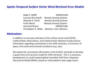
Spatio-Temporal Surface Vector Wind Retrieval Error Models Ralph F. Milliff NWRA/CoRA LucreziaRicciardulliRemote Sensing Systems Deborah K. Smith Remote Sensing Systems Frank Wentz Remote Sensing Systems Jeremiah Brown NWRA/CoRA Christopher K. WikleStatistics, Univ. Missouri Motivation: In addition to accurate estimates of the surface vector wind (SVW), scatterometer observations, and scatterometer datasets include precise information regarding uncertainties in the SVW retrievals, as functions of space, time and environmental conditions (e.g. rain). We exploit the uncertainty information in the Ku2011 retrievals to develop a space-time error process model for SVW retrievals. This is a necessary development on a path toward global ensemble SVW from a Bayesian Hierarchical Model (BHM), based on multi-platform data stage inputs.
Spatio-Temporal Error Model Parameterizations vector of scatterometer wind component obs at time Let be an vector of the “true” wind component from a prediction grid at time t Let be an associated Then a Gaussian spatial error model is: where is an matrix that maps obs to the prediction grid, is an spatial error covariance matrix, and incidence matrix for mapping errors to prediction locations is an Parameterization 1:Diagonal variance matrix Let be m-dimensional scatterometer error estimates for month j, then is a diagonal variance matrix approximation to the full covariance where is a (monthly) variance inflation parameter
Spatio-temporal Error Model parameterizations (cont’d) Parameterization 2:EOFs of error variance • Remove temporal mean variance for each x,y • Find the m x p matrix of spatial structure functions then Plan • Error estimates from monthly SOS QuikSCAT Ku2011 wind speed vs. WindsatClimo • Monthly Maps for weak ENSO warm event (WE) and neutral years • EOFs and PCs for WE and neutral time series (i.e. as in parameterization 2) • Prototype global wind BHM with spatio-temporal error model • regional (tropical Pacific), parameterization 1
SOS: Sum of Squared Differences For each cell, with i=1,N observations Where var(σobs) represents the measurement noise
Annual Average SOS in a weak ENSO Warm Event Year (2002-2003)
Error EOF and PC Calculation • Monthly diagonal variance matrix from vectorization of SOS maps • Remove temporal mean at each x,y • Singular value decomposition (lose 1 d.o.f. by removing mean) • - yields 11 EOFs and associated PCs for 12 month dataset • Compare ENSO warm event year with ENSO neutral year • - ENSO cold event year (2007-2008) roughly the same as neutral (not shown)
Error EOF and PC Comparison: Leading Modes ENSO WE and Neutral Neutral Year Warm Event Year
2005-2006 (neutral) 2002-2003 (warm event) Spatial Structure Functions: Modes 1-4
2005-2006 (neutral) 2002-2003 (warm event) Spatial Structure Functions: Modes 5-8
Principal Components: ENSO Neutral and WE years, modes 1-8 2005-2006 (neutral) 2002-2003 (warm event) 34% 33% 13% 14% 12% 12% 7% 7% 6% 6% 6% 6% 5% 5% 4% 5%
155°E to 105°W; 25°S to 25°N 392 x 200 at 0.25° Ku2011 3-day Avg L3 SVW 30d (Sep 2002)
Posterior Mean Results: 10 Sep 2002 ms-1 u(x,y) σu(x,y) missing data σu
Summary and Future Plans • Scatterometer retrievals include valuable uncertainty information for constructing • spatio-temporal error models • - useful advances in data assimilation (Kalman gain, denom Cost Function) • - required for global SVW BHM development (“surface wind ensembles”) • Parameterization 1: diagonal error variance matrix • Parameterization 2: diagonal spatial structure functions (EOFs) and PC time series • - model time dependence of leading modes; e.g. ENSO neutral vs. WE • - mixture models • Prototype regional SVW BHM for Sep 2002 • - spatially varying u std. deviation from posterior distribution (parameters) • Basis function process model structure as in spectral parts of GCMs • - e.g. Hermite polynomials in tropics • Multiplatform data stage inputs; all with specific spatio-temporal error models • - enforce k-2 spectral dependence (nested wavelets at small scales)
σ0(wind speed, polarization) A0 as a first approximation for σ0
Posterior Mean Results: 10 Sep 2002 u(x,y) σu(x,y) missing data σu