Download
1 / 31
310 likes | 399 Views
Explore various data structures including Hash Tables, Heaps, and Balanced Search Trees. Learn algorithm analysis techniques and implementations for Priority Queue ADT. Covering topics from Priority Queue operations to Binary Heaps, this course provides a detailed examination of fundamental concepts.

E N D
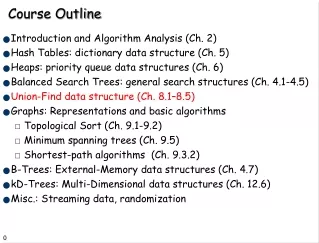
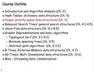
Course Outline • Introduction and Algorithm Analysis (Ch. 2) • Hash Tables: dictionary data structure (Ch. 5) • Heaps: priority queue data structures (Ch. 6) • Balanced Search Trees: general search structures (Ch. 4.1-4.5) • Union-Find data structure (Ch. 8.1–8.5) • Graphs: Representations and basic algorithms • Topological Sort (Ch. 9.1-9.2) • Minimum spanning trees (Ch. 9.5) • Shortest-path algorithms (Ch. 9.3.2) • B-Trees: External-Memory data structures (Ch. 4.7) • kD-Trees: Multi-Dimensional data structures (Ch. 12.6) • Misc.: Streaming data, randomization
Priority Queue ADT • In many applications, we need a scheduler • A program that decides which job to run next • Often the scheduler a simple FIFO queue • As in bank tellers, DMV, grocery stores etc • But often a more sophisticated policy needed • Routers or switches use priorities on data packets • File transfers vs. streaming video latency requirement • Processors use job priorities • Priority Queue is a more refined form of such a scheduler.
Priority Queue ADT • A set of elements with priorities, or keys • Basic operations: • insert (element) • element = deleteMin (or deleteMax) • No find operation! • Sometimes also: • increaseKey (element, amount) • decreaseKey (element, amount) • remove (element) • newQueue = union (oldQueue1, oldQueue2)
Priority Queue: implementations • Unordered linked list • insert is O(1), deleteMin is O(n) • Ordered linked list • deleteMin is O(1), insert is O(n) • Balanced binary search tree • insert, deleteMin are O(log n) • increaseKey, decreaseKey, remove are O(log n) • union is O(n) • Most implementations are based on heaps. . .
Heap-ordered Binary trees • Tree Structure: A complete binary tree • One element per node • Only vacancies are at the bottom, to the right • Tree filled level by level. • Such a tree with n nodes has height O(log n)
Heap-ordered Binary trees • Heap Property • One element per node • key(parent) < key(child) at all nodes everywhere • Therefore, min key is at the root • Which of the following has the heap property?
Basic Heap Operations • percolateUp • used for decreaseKey, insert percolateUp (e): while key(e) < key(parent(e)) swap e with its parent
Basic Heap Operations • percolateDown • used for increaseKey, deleteMin percolateDown (e): while key(e) > key(some child of e) swap e with its smallest child
Decrease or Increase Key ( element, amount ) • Must know where the element is; no find! • DecreaseKey key(element) = key(element) – amount percolateUp (element) • IncreaseKey key(element) = key(element) + amount percolateDown (element)
insert ( element ) • add element as a new leaf • (in a binary heap, new leaf goes at end of array) • percolateUp (element) • O( tree height ) = O(log n) for binary heap
Binary Heap Examples • Insert 14: add new leaf, then percolateUp • Finish the insert operation on this example.
deleteMin • element to be returned is at the root • to delete it from heap: • swap root with some leaf • (in a binary heap, the last leaf in the array) • percolateDown (new root) • O( tree height ) = O(log n) for binary heap
Binary Heap Examples • deleteMin. Hole at the root. • Put last element in it, percolateDown.
Array Representation of Binary Heaps • Heap best visualized as a tree, but easier to implement as an array • Index arithmetic to compute positions of parent and children, instead of pointers.
Short cut for perfectly balanced binary heaps • Array implementation Lchild = 2·parent Rchild = 2·parent+1 1 parent = child/2 3 2 4 5 6 7 9 8
Heapsort and buildHeap • A naïve method for sorting with a heap. • O(N log N) • Improvement: Build the whole heap at once • Start with the array in arbitrary order • Then fix it with the following routine for (int i=0; i<n; i++) H.insert(a[i]); for (int i=0; i<n; i++) H.deleteMin(x); a[i] = x; template <class Comparable> BinaryHeap<Comparable>::buildHeap( ) for (int i=currentSize/2; i>0; i--) percolateDown(i);
buildHeap Fix the bottom level Fix the next to bottom level Fix the top level
Analysis of buildHeap 2 15 4 10 11 5 9 13 3 6 1 12 16 17 8 7 14 18 • For each i, the cost is the height of the subtree at i • For perfect binary trees of height h, sum:
Summary of binary heap operations • insert: O(log n) • deleteMin: O(log n) • increaseKey: O(log n) • decreaseKey: O(log n) • remove: O(log n) • buildHeap: O(n) • advantage: simple array representation, no pointers • disadvantage: union is still O(n)
Some Applications and Extensions of Binary Heap • Heap Sort • Graph algorithms (Shortest Paths, MST) • Event driven simulation • Tracking top K items in a stream of data • d-ary Heaps: • Insert O(logd n) • deleteMin O(d logd n) • Optimize value of d for insert/deleteMin
Leftist heaps: Mergeable Heaps • Binary Heaps great for insert and deleteMin but do not support merge operation • Leftist Heap is a priority queue data structure that also supports merge of two heaps in O(log n) time. • Leftist heaps introduce an elegant idea even if you never use merging. • There are several ways to define the height of a node. • In order to achieve their merge property, leftist heaps use NPL (null path length), a seemingly arbitrary definition, whose intuition will become clear later.
Leftist heaps • NPL(X) : length of shortest path from X to a null pointer • Leftist heap : heap-ordered binary tree in which NPL(leftchild(X)) >= NPLl(rightchild(X))for every node X. • Therefore, npl(X) = length of the right path from X • also, NPL(root) log(N+1) • proof: show by induction that NPL(root) = r implies tree has at least 2r - 1 nodes
Leftist heaps • NPL(X) : length of shortest path from X to a null pointer • Two examples. Which one is a valid Leftist Heap?
Leftist heaps • NPL(root) log(N+1) • proof: show by induction thatNPL(root) = r implies tree has at least 2r - 1 nodes • The key operation in Leftist Heaps is Merge. • Given two leftist heaps, H1 and H2, merge them into a single leftist heap in O(log n) time.
Leftist heaps: Merge • Let H1 and H2 be two heaps to be merged • Assume root key of H1 <= root key of H2 • Recursively merge H2 with right child of H1, and make the result the new right child of H1 • Swap the left and right children of H1 to restore the leftist property, if necessary
Leftist heaps: Merge • Result of merging H2 with right child of H1
Leftist heaps: Merge • Make the result the new right child of H1
Leftist heaps: Merge • Because of leftist violation at root, swap the children • This is the final outcome
Leftist heaps: Operations • Insert: create a single node heap, and merge • deleteMin: delete root, and merge the children • Each operation takes O(log n) because root’s NPL bound
Merging leftist heaps Merge(t1, t2) if t1.empty() then return t2; if t2.empty() then return t1; if (t1.key > t2.key) then swap(t1, t2); t1.right = Merge(t1.right, t2); if npl(t1.right) > npl(t1.left) then swap(t1.left, t1.right); npl(t1) = npl(t1.right) + 1; return t1 • insert: merge with a new 1-node heap • deleteMin: delete root, merge the two subtrees • All in worst-case O(log n) time
Other priority queue implementations • skew heaps • like leftist heaps, but no balance condition • always swap children of root after merge • amortized (not per-operation) time bounds • binomial queues • binomial queue = collection of heap-ordered “binomial trees”, each with size a power of 2 • merge looks just like adding integers in base 2 • very flexible set of operations • Fibonacci heaps • variation of binomial queues • decreaseKey runs in O(1) amortized time,other operations in O(log n) amortized time