Download
1 / 27
270 likes | 288 Views
Long-Time Molecular Dynamics Simulations through Parallelization of the Time Domain. Ashok Srinivasan Florida State University http://www.cs.fsu.edu/~asriniva. Aim: Simulate for long time spans Solution features: Use data from prior simulations to parallelize the time domain.

E N D
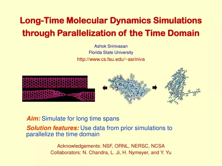
Long-Time Molecular Dynamics Simulations through Parallelization of the Time Domain Ashok Srinivasan Florida State University http://www.cs.fsu.edu/~asriniva Aim:Simulate for long time spans Solution features: Use data from prior simulations to parallelize the time domain Acknowledgements: NSF, ORNL, NERSC, NCSA Collaborators: N. Chandra, L. Ji, H. Nymeyer, and Y. Yu
Outline • Background • Limitations of Conventional Parallelization • Time Parallelization • Other Time Parallelization Approaches • Data-Driven Time Parallelization • Application to Nano-Mechanics • Application to AFM Simulation of Proteins • Conclusions and Future Work • Scaled to 1 - 3 orders of magnitude larger number of processors than conventional parallelization
Background • Molecular dynamics • In each time step, forces of atoms on each other modeled using some potential • After force is computed, update positions • Repeat for desired number of time steps • Time steps size ~ 10 –15 seconds, due to physical and numerical considerations • Desired time range is much larger • A million time steps are required to reach 10-9 s • ~ 500 hours of computing for ~ 40K atoms using GROMACS • MD uses unrealistically large pulling speed • 1 to 10 m/s instead of 10-7 to10-5 m/s
Limitations of Conventional Parallelization • Conventional parallelization decomposes the state space across processors • It is effective for large state space • It is not effective when computational effort arises from a large number of time steps • … or when granularity becomes very fine due to a large number of processors
Limitations of Conventional Parallelization • Results on scalable codes • Does not scale efficiently beyond 10 ms/iteration • If we want to simulate to a ms • Time step 1 fs 1012 iterations 1010s ≈ 300 years • If we scaled to 10 s per iteration • 4 months computing time NAMD, 327K atom ATPase PME, Blue Gene, IPDPS 2006 NAMD, 92K atom ApoA1 PME, Blue Gene,IPDPS 2006 IBM Blue Matter, 43K Rhodopsin, Blue Gene,Tech Report 2005 Desmond, 92K atom ApoA1, SC 2006
Time Parallelization • Other Time Parallelization Approaches • Dynamic Iterations/ Waveform Relaxation • Slow convergence • Parareal Method • Related to shooting methods • Not shown effective in realistic settings • Data-Driven Time-Parallelization • Use availability of prior data • Determine a relationship between current simulations and prior ones to parallelize the time domain
Other Time Parallelization Approaches Waveform Relaxation Variants • Special case: Picard iterations • Ex: dy/dt = y, y(0) = 1 becomes • dyn+1/dt = yn(t), y0(t) = 1 • In general • dy/dt = f(y,t), y(0) = y0 becomes • dyn+1/dt = g(yn, yn+1, t), y0(t) = y0 • g(u, u, t) = f(u, t) • g(yn, yn+1, t) = f(yn,t): Picard • g(yn, yn+1, t) = f(yn+1,t): Converges in 1 iteration • Jacobi, Gauss-Seidel, and SOR versions of g defined • Many improvements • Ex: DIRM combines above with reduced order modeling Exact N = 1 N = 2 N = 3 N = 4
Parareal approach • Based on an “approximate-verify-correct” sequence • An example of shooting methods for time-parallelization • Not shown to be effective in realistic situations Second prediction Initial computed result Correction Initial prediction
Data-Driven Time Parallelization • Each processor simulates a different time interval • Initial state is obtained by prediction, using prior data (except for processor 0) • Verify if prediction for end state is close to that computed by MD • Prediction is based on dynamically determining a relationship between the current simulation and those in a database of prior results If time interval is sufficiently large, then communication overhead is small
Problems with multiple time-scales • Fine-scale computations (such as MD) are more accurate, but more time consuming • Much of the details at the finer scale are unimportant, but some are • Use the course-scale response of a similar prior simulation to predict the future states of the current one A simple schematic of multiple time scales
Verification of prediction • Definition of equivalence of two states • Atoms vibrate around their mean position • Consider states equivalent if differences are within the normal range of fluctuations Mean position Displacement (from mean) Differences between trajectories that differ only due to the random number sequence in the AFM simulation of Titin
Application to Nano-Mechanics Carbon Nanotube Tensile Test • Pull the CNT • Determine stress-strain response and yield strain (when CNT starts breaking) using MD Experiments 1. CNT identical to prior results, but different strain-rate • 1000-atoms CNT, 300 K 2. CNT identical to prior results, but different strain-rate and temperature 3. CNT differs in size from prior result, and simulated with a different strain-rate Blue: Exact 450K Red: 200 processors
Dimensionality Reduction • Movement of atoms in a 1000-atom CNT can be considered the motion of a point in 3000-dimensional space • Find a lower dimensional subspace close to which the points lie • We use principal orthogonal decomposition • Find a low dimensional affine subspace • Motion may, however, be complex in this subspace • Use results for different strain rates • Velocity = 10m/s, 5m/s, and 1 m/s • At five different time points • [U, S, V] = svd(Shifted Data) • Shifted Data = U*S*VT • States of CNT expressed as • m + c1 u1 + c2 u2 u u m
Basis Vectors from POD • CNT of length 100 A with 1000 atoms at 300 K Blue: z Green, Red: x, y u1 (blue) and u2 (red) for z u1 (green) for x is not “significant”
Prediction When v is the only parameter • Static Predictor • Independently predict change in each coordinate • Use precomputed results for 40 different time points each for three different velocities • To predict for (t; v) not in the database • Determine coefficients for nearby v at nearby strains • Fit a linear surface and interpolate/extrapolate to get coefficients c1 and c2 for (t; v) • Get state as m + c1 u1 + c2 u2 • Dynamic Prediction • Correct the above coefficients, by determining the error between the previously predicted and computed states Green: 10 m/s, Red: 5 m/s, Blue: 1 m/s,Magenta: 0.1 m/s,Black: 0.1m/s through direct prediction
Verification: Error Thresholds • Consider states equivalent if difference in position, potential energy, and temperature are within the normal range of fluctuations • Max displacement 0.2 A • Mean displacement 0.08 A • Potential energy fluctuation 0.35% • Temperature fluctuation 12.5 K
Stress-strain response at 0.1 m/s • Blue: Exact result • Green: Direct prediction with interpolation / extrapolation • Points close to yield involve extrapolation in velocity and strain • Red: Time parallel results
Speedup • Red line: Ideal speedup • Blue: v = 0.1m/s • Green: A different predictor • v = 1m/s, using v = 10m/s • CNT with 1000 atoms • Xeon/ Myrinet cluster
Temperature and velocity vary • Use 1000-atom CNT results • Temperatures: 300K, 600K, 900K, 1200K • Velocities: 1m/s, 5m/s, 10m/s • Dynamically choose closest simulation for prediction Speedup 450K, 2m/s … Linear Stress-strain Blue: Exact 450K Red: 200 processors
CNTs of varying sizes • Use a 1000-atom CNT, 10 m/s, 300K result • Parallelize 1200, 1600, 2000-atom CNT runs • Observe that the dominant mode is approximately a linear function of the initial z-coordinate • Normalize coordinates to be in [0,1] • z t+Dt = z t+ z’t+DtDt, predict z’ • Speedup • - 2000 atoms • .- 1600 atoms • __ 1200 atoms • … Linear • Stress-strain • Blue: Exact 2000 atoms, 1m/s • Red: 200 processors
Predict change in coordinates • Express x’ in terms of basis functions • Example: • x’ t+Dt = a0, t+Dt + a1, t+Dt x t • a0, t+Dt, a1, t+Dt are unknown • Express changes, y, for the base (old) simulation similarly, in terms of coefficients b and perform least squares fit • Predict ai, t+Dt as bi, t+Dt + R t+Dt • R t+Dt = (1-b)R t + b(ai, t- bi, t) • Intuitively, the difference between the base coefficient and the current coefficient is predicted as a weighted combination of previous weights • We use b = 0.5 • Gives more weight to latest results • Does not let random fluctuations affect the predictor too much • Velocity estimated as latest accurate result known
Application to AFM Simulation of Proteins • Example System: Muscle Protein - Titin • Around 40K atoms, mostly water • Na+ and Cl- added for charge neutrality • NVT conditions, Langevin thermostat, 400K • Force constant on springs: 400kJ/(mol nm2) • GROMACS used for MD simulations
Prediction • Use prior results with higher velocity • Trajectories with different random number sequences • Predict based on prior result closest to current states • Use only the last verified state • Use several recent verified states • Fit parameters to the log-Weibull distribution • (1/b) e (a-x)/b-e (a-x)/b • Location: a = 0.159 • Scale: b = 0.0242
Speedup Speedup: Green - spatial on Xeon/Myrinet at NCSA,Blue - spatial on Opteron/GigE, Red - time, at NCSA Speedup with combined space (8-way) - time parallelization Green: Conventional parallelization • One time interval is 10K time steps, 5 hours sequential time • The parallel overheads, excluding prediction errors, are relatively insignificant • Above results use last verified state to choose prior run • Using several verified states parallelized almost perfectly on 32 processors with just time parallelization
Validation Spatially parallel Time parallel Mean (spatial), time parallel Experimental data
Typical Differences RMSD Solid: Between exact and a time parallel runs Dashed: Between conventional runs using different random number sequences Force Dashed: Time parallel runs Solid: Conventional runs
Conclusions and Future Work • Conclusions • Data-driven time parallelization promises substantial improvement in scalability, especially when combined with conventional parallelization • More effective in hard matter simulations • Obtained granularity of 13.5 s per iteration in one simulation • Promising for soft matter simulations too • Future Work • Better prediction • Satisfy detailed balance • References • See http://www.cs.fsu.edu/~asriniva/research.html