Download
1 / 14
160 likes | 358 Views
Lecture 7: Unsteady Laminar Flow. Impulsive Shearing Motion of a Plane Wall Laminar Boundary Layers. Impulsive shearing motion of a plane wall. At , the wall is impulsively set into motion. Non-steady plane-parallel flow:. Governing equation:. i.c .: b.c .:. (1).

E N D
Lecture 7: Unsteady Laminar Flow • Impulsive Shearing Motion of a Plane Wall • Laminar Boundary Layers
Impulsive shearing motion of a plane wall At , the wall is impulsively set into motion. Non-steady plane-parallel flow: Governing equation: i.c.: b.c.: (1) (diffusion equation) We seek solution in the form:
Finally (substituting the above partial derivatives into equation (1)), b.c.: First integration: Second integration:
Applying the first boundary condition: Applying the second boundary condition: Final expression: error function (a tabulated function) is typical thickness of the fluid layer involved into motion, it is called the thickness of the laminar boundary layer
Velocity profile for water ( ) for t=1s (green curve), 100s (red), and 10000s (brown). Videos: http://www.youtube.com/watch?v=jx8j2OVZKjc http://www.youtube.com/watch?v=TADz6fqfXo0http://www.youtube.com/watch?v=6WiplPYOv6M
Friction force Friction force exerted by the fluid and applied to the wall,
Laminar boundary layers if Conclusion: Re>>1 is typical for most engineering flows: where the flow may be separated into two regions: (i) thin viscous boundary layer and (ii) inviscid bulk flow. Comment: for very high Re( , for a flow above a plane wall), the boundary layer becomes turbulent.
Lecture 8: Irrotational (or potential) flow • Irrotational motion. Kelvin circulation theorem • Laplace equation • Bernoulli’s equation
Irrotational motion -- definition of vorticity The flow is irrotationalif for every point. The irrotational flow is always inviscid; i.e. Re>>1, but not turbulent and far from the boundaries where the viscous laminar layers are formed.
Kelvin circulation theorem Consequence of the Kelvin’s circulation theorem: if for a fluid particle, at initial moment, vorticity is zero, the vorticity remains zero for an entire trajectory of a particle (for every point on a streamline). Typical example of an irrotational flows is depicted above. This is the flow around a stationary body immersed in a fluid (the flow must be uniform at the initial moment) or the motion of a body in a stationary fluid. The flow is irrotational only at distances of several viscous boundary layers from the immersed body.
Laplace equation Governing equations for an inviscid incompressible fluid subject to gravity field: Considered flows are irrotational, i.e. . Any vector field with can be represented as gradient of a scalar, . φ is the velocity potential. Let us rewrite the governing equations in terms of velocity potential. Continuity equation turns into -- Laplace equation
Boundary conditions Solutions of the Laplace equation determine the velocity potential, hence, the velocity field. The boundary conditions are needed to find a solution. Rigid wall: the fluid is inviscid, the no-slip boundary condition cannot be satisfied. The no-slip condition is replaced by a no-penetration boundary condition. vn=0 is imposed on the wall (in terms of the velocity potential, ). Free surface: pressure is equal to the atmospheric pressure. At infinity: the velocity field must be bounded.
Bernoulli’s equation The Navier-Stokes equation turns into or -- Bernoulli’s equation As the velocity field is already determined by the Laplace equation, this equation can be used to find the pressure.
Daniel Bernoulli (Groningen, 8 February 1700 – Basel, 8 March 1782) was a Dutch-Swiss mathematician and was one of the many prominent mathematicians in the Bernoulli family. William Thomson, 1st Baron Kelvin (or Lord Kelvin), (26 June 1824 in Belfast – 17 December 1907 in Largs) was a mathematical physicist and engineer. Pierre-Simon, marquis de Laplace (23 March 1749 – 5 March 1827) was a French mathematician and astronomer whose work was pivotal to the development of mathematical astronomy and statistics. Lord Kelvin: "Heavier-than-air flying machines are impossible.“(1895)