Download
1 / 23
230 likes | 399 Views
GOCE Gravity field error variances-covariances and the related tools Example with a recent solution. G. Balmino, S. Bruinsma, J.C. Marty CNES - GRGS, Toulouse (France). ESA Living Planet Symposium 2010 Session 3.3.3. "GOCE in Geophysics". Bergen, June 27 - July 2, 2010. 1. Rationale

E N D
GOCE Gravity field error variances-covariances and the related tools Example with a recent solution G. Balmino, S. Bruinsma, J.C. Marty CNES - GRGS, Toulouse (France) ESA Living Planet Symposium 2010 Session 3.3.3. "GOCE in Geophysics" Bergen, June 27 - July 2, 2010
1. Rationale 2. Overview of method 3. Examples with a GOCE solution
1 RATIONALE
GOAL q is any geodetic function such as : - geoid heights - free-air gravity anomalies g - gravity disturbances - radial gravity gradient - vertical gradient of g - equivalent water height (with load effect), ... represented by a SH series : Clm, Slm are the coefficients of a global geopotential model, of variance-covariance matrix (N : normal matrix of the least squares adjustment of the coef. from observations) The flm's depend on the type of q, and may include spectral filtering (or tapering) coefficients, -smoothing factors for mean values - in such case Plm is replaced by its integral IPlm over a cell. Compute 2 (q) at any point P, or cov (q1 , q2 ) for two points P1, P2
2 (q) , cov (q1 , q2 ) study and use oferror patterns - geographic distribution of variances not sufficient for some applications - cross (co)- variances give finer information on anisotropies Ex : error covariances between central point and surrounding points (geoid height, gravity anomaly, eq. water height, ...) the dream !
MSS SST global geoid model h(MSS) h(GS) h0(GS) true geoid surface(GS) reference ellipsoid EXAMPLES IN OCEANOGRAPHY (i) Sea surface slopes (cf. Haagmans et al., 1991; 2000) SST = h (MSS) – h (GS) = h (MSS) – h0(GS) – h(GS) , h0 : global model ( deg. L ) h : omission ( deg. > L ) Assuming all components are uncorrelated, we have : the error variance on the SST at any point A : 2(SSTA) = 2[h(MSS)A] + 2[h0(GS)A] + 2[h(GS)A] the error variance on the slope between two points (A,B) : 2(SSTB – SSTA) = 2[h(MSS)A] + 2[h(MSS)B] – 2 cov [h(MSS)A, h(MSS)B] + 2[h0(GS)A] + 2[h0(GS)B] – 2 cov [h0(GS)A, h0(GS)B] + 2[h(GS)A] + 2[h(GS)B] – 2 cov [h(GS)A,h(GS)B] from empirical var.-covar. model
(ii) Covariances of the geoid model induced error on the geostrophic currents (Balmino; 2000, 2009) Part corresponding to vertical deflection : , y x scale : m/s
2 OVERVIEW OF METHOD
The computation of variances and covariances in "GUT" • Yk: vector of the base functions values at grid point Pk(or their integrals), • including factors flm • : full covariance matrix (lower triangle, completed to square), in core (if small) or on disc Technique: Compute these quantities on a equi-angular grid by using the exact (full) covariance matrix, , of the S.H. coefficients ( Clm , Slm ) derived from the mission data analysis 2 (q1,2) 2 (Pij ) cov (q1, q2) cov (Pij,Phk) Difficulty: is large ( ~ 40 0002 to 65 0002 , possibly ~ 100 0002 to 200 0002 in near future) Then : for any point P (any two points P1, P2), interpolate values from grid
j lat. (i) The computation of cov (Pij, Phk)is limited to distances of : Hnodes in latitude Knodes in longitude h H - Grid nodes can be at corners of equiangular cells or at their center - H and K given compute i such that i-H h i+H and j-K k j+K k - Use of symmetries : - Continuity ensured in and through the poles lon K - Simultaneous computation of tables of isotropic, N-S and E-Wcovariance functions over the zone enables the evaluation of the covariances beyond a maximum distance D(H,K) Then (for graphic display or interpolation): efficient algorithm to extract windows of covariances with respect to nodes (i,j ), i.e. to provide all for nodes (h,k) verifying i-H h i+H and j-K k j+K . Algorithms and peculiar features Ref : "Efficient propagation of error covariance matrices of gravitational models. Application to GRACE and GOCE "; G. Balmino (JoG, 2009) (ii) The computation of 2 (q)at node Pijis much simpler (indeed performed at each node with no restriction)
Algorithms key points Summation of HS series (scalar products) : first on order (m), then on degree (l) Computation of Legendre functions : stable recursive formulas with m fixed Computation of definite integrals of Legendre functions : Gerstl 's formulation (1980), modified by Balmino (1994) PSLR (Partial Sums - Longitude Recursions) technique (W. Bosch, 1983 ): - partial sums on degree (m fixed), constant for a given latitude (with Horner scheme as in Holmes & Featherstone, 2002) - longitude recursions on the grid nodes to do the sums on l , equivalent to FFT approach (O. Colombo , 1981; N. Sneeuw & R. Bun, 1996; R. Haagmans & Van Gelderen, 1991), ... but easier to implement
Interpolation procedure cov (z, v) : double bilinear interpolation of the gridded values cov (Pij , Phk ) Window of z Studied Zone Zone envelope
3 EXAMPLES WITH A GOCE SOLUTION
EXAMPLE The combined gravity field EIGEN-GOCE14p model ( CNES-GFZ solution ) Clm, Slm to degree/order 240 71 days of data : . GOCE-SST : todegree/order 110 (relative weight 0.05) . GOCE-SGG "XX + YY" (relative weight 0.5) + "ZZ" : to degree/order 240 [100 sec – 8 sec] band pass filter for all three SGG components Spherical cap regularization to compensate the polar gaps: based on EIGEN-51C to degree/order 240 Combined gravity field EIGEN-51Cmodel (to be published) combined global gravity field model to degree/order 359 • 6 years of CHAMP + GRACE (Release 4, Oct 2002 … Sept 2008) • terrestrial data: DNSC08 global gravity anomaly grid • combination based on (full) normal equations
: cumulated Kaula signal (solution) 6 cm meter 8.5 cm l Degree Geoid height signal and errors () per degree Solution EIGEN-GOCE-14p
degree l order m Slm Clm ERRORS IN THE SPECTRAL DOMAIN sectorials sectorials zonal SH
ERRORS IN SPACE DOMAIN Solution EIGEN-GOCE-14p Geoid height error [cm] from the var/cov matrix to d/o 240 (1° x 1° grid) cm 6 5 7 8 9 10
COVARIANCES Solution EIGEN-GOCE-14p 20°N , 80°N 60°W , 30° E Example of computation over a large area : Z (H) = 20° ; (K) = 20° E(Z) : zone envelope (goes over the pole) (Z) window of P P Full model : to degree/order 240
EXAMPLES OF COVARIANCES IN TEST AREA : 3 WINDOWS Solution EIGEN-GOCE-14p (to d/o 240) 3.0 70 80 50 2.5 2.0 40 60 70 1.5 1.0 30 0.5 50 60 0.0 -0.5 20 50 40 -1.0 -1.5 10 40 30 -2.0 10 20 30 40 0 -10 -60 -50 0 -40 -30 -20 -20 -30 Geoid heights covariances - unit = cm2
GEOID heights covariance functions 7.8 cm covariances in cm2 different y-scale ! distance (degree)
Geostophic velocity error ellipses : ( , ) part Solution EIGEN-GOCE-14p 50 40 latitude 30 -80 -60 -70 -50 -40 -30 longitude velocity (Levitus) radius : 1 cm/s scales 10 cm/s
CONCLUSION With only 71 days of GOCE data, it has been possible to characterize the errors associated with the spherical harmonic coefficients of a global gravity model (EIGEN-GOCE-14p) derived from these data. In particular the mapping of the covariances in the space domain exhibits a remarkable isotropy, and the prospects for oceanographic applications look very promising.