27. The Structure of the Universe Goals :

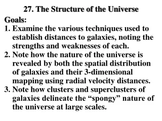
1. 27. The Structure of the Universe Goals: 1. Examine the various techniques used to establish distances to galaxies, noting the strengths and weaknesses of each. 2. Note how the nature of the universe is revealed by both the spatial distribution of galaxies and their 3-dimensional mapping using radial velocity distances. 3. Note how clusters and superclusters of galaxies delineate the “spongy” nature of the universe at large scales.

2. The Extragalactic Distance Scale: The techniques for measuring distances to galaxies are varied, each depending directly or indirectly upon a local calibration of distances tied to trigonometric parallaxes for stars and/or star cluster main-sequence fitting. Measurement of trigonometric parallaxes has a long and colourful history that continues to the present. The Hipparcos mission (mid ’90s) was intended to supplant the old technique of measuring absolute parallaxes for stars through the intermediary of relative parallaxes, but has run afowl of systematic errors of its own, not admitted by team members. The same problems may also continue with the Gaia mission. Hipparcos parallaxes have a magnitude limit near 10, not so Gaia, which has a bright limit, meaning that many important types of stars are not on the program of observation. The technique of calibrating distances using open cluster main-sequence fitting has been more reliable overall.

3. How are distances to galaxies determined? Distances to nearby solar system objects are measured by radar, nearby stars by parallax, then cluster main sequence fitting, the Cepheid PL relation, and finally Type Ia supernovae.

4. The standard candles used to measure distances to galaxies are: For “nearby” galaxies, Cepheid variables, since their periods of pulsation correlate with their intrinsic luminosities (period-luminosity relation). (similar to using the “watts” label on a light bulb to determine how bright it is) For distant galaxies, Type Ia supernovae, since their peak brightness is always the same. They are also the brightest class of supernovae. (similar to, say, all supernovae appearing as bright as a “150 watt” light bulb)

5. Determining distances to galaxies using Cepheid variables. Step 1. Identify a Cepheid from its changes in brightness with time. Step 2. Measure its mean brightness and period of variability. Step 3. Use the Cepheid period-luminosity relation to establish its intrinsic brightness and calculate its distance.

6. A review of classical Cepheids, their properties and usefulness as distance indicators, is given by Turner (2012, JAAVSO, 40, 502). Note how reliably the PL relation is defined by current calibrators for Cepheids with reliable reddenings (points) or with cluster or HST parallaxes (plus signs).

7. Evidence for a robust calibration of the Cepheid period-luminosity relation from cluster Cepheids is seen in the figures. Cluster Cepheids and Cepheids with Parallaxes from the Hubble Space Telescope (old style and solid) define the same PL relation.

8. Evidence for a systematic error in Hipparcos parallaxes for Cepheids is also seen. The cluster PL calibration’s validity is demonstrated by the fact that it matches the distance to the galaxy NGC 4258 found geometrically from masers. Cepheid distances generally use a Wesenheit (reddening-free) relation rather than PLC (period- luminosity-colour) relation.

9. Reddening-Free Indices are sometimes used in Galactic studies. If the extinction law is invariant throughout the Galaxy with no curvature term, then EU–B/EB–V = X, a constant. Johnson & Morgan (ApJ, 117, 313, 1953) introduced a Q parameter for the UBV system that took advantage of this invariance property, namely: Note that Q is defined the same way in terms of either reddened or intrinsic colours. But X is NOT constant.

10. In similar fashion one can define a special function for Cepheids that removes differences in reddening, namely: which is also the same when defined using either observed or reddening-corrected colours and magnitudes. Sidney van den Bergh created a W-function with R being the colour term in the PLC relation. It behaves in similar fashion. The function above, created by Barry Madore, is referred to by him as a Wesenheit function.

11. A typical Wesenheit formula, updated as of 2014, is: where the < > brackets denote intensity means of the corresponding magnitudes. Tests done for the galaxy NGC 4258 indicate that the scatter in the WV−log P relation reaches a minimum for RV = 3.0. That is consistent with extinction towards the Galactic halo.

12. The Wesenheit function applied to NGC 4258 with RV = 3.0 yields a distance modulus of 27.489 (figure). Cepheid calibrators are plotted in black, Cepheids in the outer regions of NGC 4258 in red, and Cepheids in its inner regions, likely contaminated, in green. A larger distance for the calibrating galaxy NGC 4258 leads to a value for the Hubble constant H0 of order 65 km s−1 Mpc−1, differing from 74.3 ±2.1 km s−1 Mpc−1 by the Carnegie Hubble team, but consistent with 67.3 ±1.2 km s−1 Mpc−1 by the Planck team.

13. Wilson-Bappu Effect. The Wilson-Bappu effect is a direct correlation between the luminosity of a star and the width of the central emission core of the single-ionized calcium K-line in late-type stars (spectral types G and K). Since it appears to apply to bright giants as well as dwarfs, it spans a large range of luminosity. The relationship is typically calibrated using parallaxes, but is much less accurate (typically ±0.6 magnitude) than cluster main-sequence fitting, so sees very limited applications in calibration work. The central emission reversal in Ca II K-line cores originates in optically-thin spectral lines from overlying chromospheric gas. The Wilson-Bappu effect is used to calibrate the distance to the Hyades cluster, which contains a few GK giants, and therefore to solidify the cluster ZAMS distance scale.

14. The Cepheid Distance Scale. Despite the solid nature of the calibration of the Cepheid PL relation, problems still arise. The manner of extracting photometric magnitudes for crowded stars in distance galaxies is not without criticism, and many existing relationships rely upon Magellanic Cloud Cepheids as calibrators rather than Galactic calibrators. The Galactic calibration of the Cepheid PL relation is supported not only by HST parallaxes and cluster parallaxes, but also by calibrations tied to the Baade-Wesselink method, which uses Cepheid photometry in combination with radial velocity variations to deduce Cepheid luminosities directly. Magellanic Cloud Cepheid suffer from two problems: (i) an uncertain distance to the LMC (the best current distance modulus is 18.43), and (ii) an uncertain metallicity dependence on Cepheid luminosities (which may be unimportant). Galactic Cepheids have metallicities like those in nearby spiral galaxies, whereas LMC Cepheids are metal-poor.

15. RR Lyrae Variables and Type II Cepheids. These types of “Cepheids” are lower-mass (0.5-2.0 M) pulsators that also appear to obey a PL relation, but one that is less luminous than that for classical Cepheids. Their lower luminosities reflect their origin from older, often metal-poor, lower-mass stars, but it also means that they are more difficult to detect than classical Cepheids in nearby galaxies. Often they are simply ignored. But see the recent work of Dan Majaess on a calibration of the PL relation for Type II Cepheids, and how it confirms the distances to nearby galaxies established from classical Cepheids. The variables are often detected in the same surveys of nearby galaxies made to measure the brightness changes of their classical Cepheids, and a number of other researchers have begun to make use of them as secondary distance calibrators for the sample of Cepheid calibrating galaxies.

16. Type II Cepheids in nearby galaxies, taken from published observations of variable stars in the galaxies by Dan Majaess. In each case the upper two relations represent expectations for classical and overtone Cepheids, while the lower line represents a Wesenheit relation for Type II Cepheids. Note that some Type II Cepheids have pulsation periods as long as some classical Cepheids, and are about as luminous. Their potential as standard candles for the extragalactic distance scale is very real.

17. M Supergiants and Type C Semiregular Variables. These stars are pulsating M supergiants with periods often in excess of 1-2 years. Yet they also appear to obey a PL relation (green pts in graph), making them particularly valuable as distance candles. They are more luminous than Cepheids, and are apparently more numerous in spiral galaxies, but little work has been done to use them as calibrators.

18. M supergiants saw use as distance indicators differently 30 years ago when stellar evolutionary models by the Geneva group revealed that very massive stars (M > 25 M) never make it to the red side of the HR diagram during post-main-sequence evolution. Humphreys noted an upper limit for M supergiant luminosities near MV = –8.0 (Mbol = –9.7), which can be used as a standard candle provided that either photometry or spectroscopy is available for the brightest stars in a galaxy to identify the M supergiants (B–V ~ 1.7).

19. See HR diagram for the open cluster Trumpler 37 below. The cluster must have V0−MV 10, since A0 ZAMS stars [(B−V)0 = 0.00] have MV = +1.56. The red supergiant μ Cep (top right of diagram), a member that is the most luminous pulsating red supergiant, must have MV −8.0.

20. H II Regions. Sandage and Tammann expended considerable effort to establish the diameters of H II regions as a standard candle 40 years ago, but the technique was never particularly reliable. The diameter of an H II region depends in a complicated fashion on the masses of the stars in the driving cluster at its core as well as its ages (older H II regions have had time to expand) and the density of gas in its surroundings. The technique has died out in recent years, which is probably a good thing. There is an obvious limit to its usefulness as a standard candle in any event, since the H II region must be resolved as such for the technique to apply.

21. Type Ia Supernovae. There are several different types of supernovae, distinguishable by differences in their light curves and the spectral lines they display near maximum light. The spectral features and light curve shapes have been organized over the years into types I and II, where type I supernovae lack hydrogen lines and Type II do contain hydrogen lines. Subtypes are recognized by differences in their light curves or spectra, and are summarized below: Supernova Type Spectra Ia Lacks H and displays a Si II line at 615.0 nm near peak light Ib He I line at 587.6 nm and no Si II line at 615 nm Ic Weak or no He lines and no Si II line at 615 nm IIP Reaches a “plateau” in its light curve IIL Displays a “linear” decrease in its light curve Type II supernovae are the expected terminal stage in the evolution of massive stars, while Type I supernovae may have a variety of origins. Type Ia supernovae are the objects of interest as extragalactic distance indicators.

22. Several means exist for creating Type Ia supernovae. All share a common underlying mechanism, deflagration of a CO white dwarf bumped over the Chandrasekhar limit (~ 1.38 M for a non-rotating star) through mass accretion in a close binary system. The CO white dwarf is no longer able to support itself through electron degeneracy pressure and begins to collapse. Many believe the upper mass limit is not formally attained. Increasing temperature and density inside the core ignite carbon fusion as the star approaches the limit (to within about 1%) before collapse is initiated. Within a few seconds, a substantial fraction of the star’s matter undergoes nuclear fusion, releasing enough energy (1–2 × 1044 J) to unbind the star in a supernova explosion. An outwardly expanding shock wave is generated, reaching velocities of order 5,000–20,000 km/s, ~0.03c. A significant increase in luminosity occurs, the supernova reaching an absolute magnitude of –19.3 with little variation. The last property is what makes them so valuable as distance indicators.

23. In order to be used as a distance indicator, a Type Ia supernova must first be identified as such (spectroscopy), then it must be followed photometrically in order to establish a reasonably complete light curve. Maximum light for the supernova may have been unobserved, but the light curve is regular enough that the time of light maximum can usually be established reliably.

24. Light curve shape for Type Ia supernovae in different wavebands, and the relationship between decline rate and maximum luminosity. Templates are frequently used to match the light curve in order to attain a best fit overall.

25. Example (textbook). The Type Ia supernova SN 1963p in the galaxy NGC 1084 had an apparent blue magnitude of B = 14.0 at maximum light. Calculate the distance to the supernova for an extinction of AB = 0.49. (B – AB) – MB = 5 log d – 5 , so log d = (B – AB– MB + 5)/5 = (14.0 – 0.49 + 19.3 + 5)/5 = 37.81/5 = 7.562 So d = 107.562 = 36.5 Mpc So why does the textbook give 41.9 Mpc???

26. Novae. Novae are less luminous than supernova and originate differently, enough to produce a range of luminosities at light maximum. They are also created in close binary systems when a compact white dwarf accumulates mass from its companion. In the case of novae, the white dwarf is not near the Chandrasekhar limit and the accreted gas undergoes thermonuclear burn-off near the surface of the white dwarf. More massive white dwarfs are also smaller, producing greater compression of the accreted mass and a hotter, briefer explosive response that produces a brighter nova of shorter duration. There is a moderately tight relation between Mmax and rate of decline first noted by Arp in 1956 for M31 novae. They are roughly as luminous as the most luminous Cepheids.

27. Globular Cluster Luminosity Functions. This technique was described previously in Chapter 25, and has been used as a secondary means of establishing distances to galaxies as distant as the Virgo cluster. Application of the technique involves fitting a Gaussian profile to counts of globular clusters as a function of apparent magnitude, using the derived width and location of maximum of the fitted profile to deduce both the richness of the globular cluster population for the galaxy and its distance modulus relative to the maximum derived for Milky Way globulars. Of course the globulars must first be distinguished from stars. Application to Virgo cluster galaxies by Harris is indicated in the figure.

28. Planetary Nebulae Luminosity Functions. Evolutionary tracks are displayed for stars evolving from the asymptotic giant branch (AGB) through the central star of planetary nebula (PN) stage, for M = 0.535, 0.569, 0.597, 0.633, 0.677, 0.754, and 0.900 M (bottom to top), compared with the location of actual central stars of PN. At the high mass end the evolution is too fast to permit creation of a PN. The most probable mass is ~0.6-0.7 M, typical of white dwarfs.

29. The upper luminosity limit is also seen in the maximum luminosities of the PNe themselves, and can be used as a distance indicator, as indicated here for M31 and Leo group PNe. The PNe are detected through narrow band photometry and then counted as a function of magnitude. The luminosity cutoff is well-defined, and PN distances compare well with Cepheid distances. PNe have also been used to estimate the distance to the Galactic centre.

30. Surface Brightness Fluctuation Method. Surface brightness fluctuation (SBF) is a secondary distance indicator used to estimate distances to galaxies. The technique uses the fact that galaxies are made up of a finite number of stars. The number of stars in any small patch of the galaxy will vary from point to point, creating a noise-like fluctuation in the surface brightness distribution. While the various stars present in a galaxy will cover an enormous range in luminosity, the SBF can be characterized as if all stars had the same brightness, which is the luminosity-weighted integral over the luminosity distribution of stars. Older elliptical galaxies have fairly consistent stellar populations, thus the typical “fluctuation star” closely approximates a standard candle. In practice, corrections are required to account for variations in age or metallicity from galaxy to galaxy.

31. The SBF pattern is measured from the power spectrum of the residuals left behind from a deep galaxy image after a smooth model of the galaxy has been subtracted. The SBF pattern is evident as the transform of the point spread function in the Fourier domain. The amplitude of the spectrum gives the luminosity of the fluctuation star. Since the technique depends on a precise understanding of the image structure of the galaxy, extraneous sources such as globular clusters and background galaxies must be excluded from the analysis, as well as areas of interstellar dust absorption. In practice it means that SBF works best for elliptical galaxies or the bulges of S0 galaxies, since spiral galaxies generally have complex morphologies and extensive dust features. SBF is calibrated by use of fiducial Cepheid Period-Luminosity relation (P-L) based on observations of variables located in the Large Magellanic Cloud (Tonry 1991).

32. An example of the surface brightness fluctuation technique applied to galaxies in various cluster groups, including the Local Group. Note that the relationship has a distinct shape for galaxies of comparable distance.

33. The Tully-Fisher Relation. The Tully-Fisher relation was introduced in Chapter 25. Its application to the determination of distances to spiral galaxies requires a calibration, usually using galaxies whose distances are established using Cepheids or other techniques. Note that any recalibration of distances to the calibrating galaxies affects secondary techniques like the TF relation. The TF relation in various passbands is illustrated at right.

34. The D-σ Relation. The Faber-Jackson relationship, which expresses the power-law correlation between an elliptical galaxy’s luminosity and its internal velocity dispersion, was also introduced in Chapter 25. The technique displays considerable scatter (see figure at right), however, so a modification has been developed in recent years that is referred to as the D-σ relation.

35. Two groups conducting surveys of elliptical galaxies arrived independently at a new result: the FJ correlation could be tightened considerably by the addition of a third parameter, namely surface brightness. In its modern incarnation, the new correlation has become known as the Dn-σ relation: a power-law correlation between the luminous diameter Dn and the internal velocity dispersion σe, namely: where γ = 1.20 ±0.10 according to some researchers. More broadly, the Dn-σ relation and its variants may be viewed as manifestations of the Fundamental Plane (FP) of elliptical galaxies, a planar region in the 3-dimensional space of structural parameters in which normal ellipticals are found. One expression of the FP relates effective diameter to internal velocity dispersion and central I-band surface brightness: where α = 1.44 ±0.04 and β = 0.79 ±0.04.

36. Two versions of the Fundamental Plane for Virgo cluster and Coma cluster elliptical galaxies.

37. Brightest Galaxies in Clusters. Studies of clusters of galaxies (e.g. Schechter 1976) indicate that the magnitude of the brightest galaxy in a cluster, or better yet, the 10th brightest galaxy in a cluster, is tightly constrained in luminosity, hence making it a good distance indicator. For 10 nearby clusters, <MV> = −22.83 ±0.61 for the brightest galaxy.

38. The technique has become more sophisticated in recent years (see below), although less complicated versions can be just as reliable. Below is the Hubble diagram for the Lauer & Postman (1992) BCG sample. Apparent magnitude within rm is plotted against log redshift. The straight line plotted through the points has slope 5, the relation expected for a linear Hubble flow.

39. An example of a calibration of m10 (magnitude of the 10th brightest cluster galaxy) versus log redshift (z) for some galaxy surveys (lower left), and how that translates into a study of galaxy cluster ellipticity e as a function of implied redshift z (lower right). Note how more distant galaxy clusters tend to be less spherically symmetric than nearby galaxy clusters.

40. Eclipsing Binaries. In 1994 a group including Ed Guinan (Villanova) proposed the use of extragalactic eclipsing binaries with well-determined physical properties as standard candles to improve the extragalactic distance scale. The advent of high quantum efficiency/low noise CCDs makes it possible to obtain high precision light and radial velocity curves for the more luminous OB-type eclipsing binaries in the Magellanic Clouds with even small to moderate size (1–2m) telescopes. That can lead to the determination of distance moduli (m-M)0 to the LMC and SMC with precisions of about ±0m.15 for individual binaries. The distances are essentially free from the assumptions made using other distance indicators. The technique makes use of Wilson-Devinney code models for eclipsing binaries, but is otherwise independent of parallax and proper motion data.

41. Application of the technique to an eclipsing OB system in M33 by Bonanos et al. (2006). Note precision of ±0m.12, after correction for reddening.

42. Gravitational Lens Time Delay and H0. When a quasar is viewed through a gravitational lens, multiple images are seen. The light paths from the quasar that form the images have different lengths that differ by approximately d(cos θ1 – cos θ2) where θs are the deflection angles and d is the distance to the quasar. Since quasars are time variable sources, the path length difference can be measured by looking for a time-shifted correlated variability in the multiple images. By 1996 the time delay had been measured in 4 quasars, giving H0 = 63 ±12 km/s/Mpc, H0 = 42 km/s/Mpc, although another analysis of the same data gave H0 = 60 ±17 km/s/Mpc, H0 = 52 ±11 km/s/Mpc, H0 = 63 ±15 km/s/Mpc, and H0 = 71 ±20 km/s/Mpc.

43. The time delay in separate images A and B of the double QSO 0957+561.

44. The more usual form of gravitational lensing by a rich cluster of galaxies.

45. Sunyaev-Zel’dovich Effect and H0. Hot gas in clusters of galaxies distorts the spectrum of the cosmic microwave background observed through the cluster. The hot electrons in a cluster scatter a small fraction of the cosmic microwave background photons and replace them with photons of slightly higher energy. The difference between the CMB seen through the cluster and the unmodified CMB seen elsewhere on the sky can be measured. Actually only about 1% of the photons passing through the cluster are scattered by the electrons in the hot ionized gas in the cluster, and those photons have their energies increased by an average of about 2%. That leads to a shortage of low energy photons of about 0.010.02 = 0.0002 or 0.02%, which gives a decrease in the brightness temperature of ~500 mK. At high frequencies (≥ 218 GHz) the cluster appears brighter than the background. The effect is proportional to the number density of electrons, the thickness of the cluster along the line of sight, and the electron temperature.

46. The parameter that combines those factors is called the Kompaneets y parameter, y = τ(kT/mc2), where τ is the optical depth or the fraction of photons scattered, while (kT/mc2) is the electron temperature in units of the rest mass of the electron. The X-ray emission IX from the hot gas in the cluster is proportional to the square of the number density of electrons, the thickness of the cluster along our line of sight (LOS), and the electron temperature and X-ray frequency. As a result, the ratio: y2/IX = constant  (Thickness along LOS) f(T) If the thickness along the LOS is assumed to be the same as the diameter of the cluster, the observed angular diameter can be used to find the distance. The technique is very difficult, but recent work with closely packed radio interferometers operating at 30 GHz has given precise measurements of the radio brightness decrement for 18 clusters; only a few have adequate X-ray data. A recent Sunyaev-Zeldovich determination of the Hubble constant gave 77 ±10 km/s/Mpc from 38 clusters.

47. The Virgo cluster of galaxies.

48. Distance Indicator Summary

49. The Expansion of the Universe: With the distances to nearby galaxies established via the various techniques outlined in the previous section, with highest weight to those using the Cepheids and Type Ia supernovae, it is found that there is a correlation of the Doppler shift of a galaxy’s spectrum with distance. The effect was first noted by Slipher in 1914, but was later elaborated upon by Hubble in 1929 and by Hubble and Humason in 1934. The relationship is linear for nearby galaxies, and corresponds to an increase in a galaxy’s velocity of recession v with increasing distance d. Known as the Hubble Law, it is generally described as: where H0 is the Hubble constant , always cited in units of km/s per Mpc, i.e. km s–1 Mpc–1. Typical current values have been found to lie in the range 50–100 km s–1 Mpc–1, with “best” values lying around 72 km s–1 Mpc–1.

50. Redshift-Distance Relation. Cluster elliptical galaxies of different redshift, and how that correlates with distance (distances recalibrated for figure at right).