Download

1 / 20
200 likes | 324 Views
More Detail for a Combined Timing and Power Attack against Implementations of RSA Werner Schindler Werner.Schindler@bsi.bund.de Colin D. Walter Colin.Walter@comodogroup.com. Overview. History. Montgomery’s Mod Mult Algorithm Assumptions Output Distributions

E N D
More Detail for a Combined Timing and Power Attack against Implementations of RSA Werner Schindler Werner.Schindler@bsi.bund.de Colin D. Walter Colin.Walter@comodogroup.com
Overview • History • Montgomery’s Mod Mult Algorithm • Assumptions • Output Distributions • Distinguishing Secret Exponent Digits • Simulation Results • Counter-Measures • Conclusion
History • Kocher et al (1996,1997): Timing and Power Attacks on smart cards – the concepts. • Dhem et al (1998): Initial stats on observed data. • Walter & Thompson (2001): Theoretical explanation. • Schindler (2002): Statistical detail when distributions can be computed. • Here: Treating mod multn and expn algorithms which may be used in practice.
Timing and power attacks – basic ideas I(t) ti (measured running time) t Timing attacks exploit time differences needed for various input values. Power attacks exploit the power consumption. Visa 4527 6604 9152 4560 WALTER SCHINDLER Expires 12/2003 yi yid (mod M)
Montgomery Modular Multiplication Notation: r = base of representation; R = rn= Montgomery factor. • { Pre-condition: 0 £A < R = rn } P ¬ 0 ; For i ¬ 0 to n-1 do Begin q ¬ (p0+aib0)(–m0–1) mod r ; P ¬ (P + aiB + qM) div r ; End ; { Post-conditions: PrnºA×B mod M , ABr–n£P < M + ABr–n } If P ≥ Mthen P ¬ P–M ; ________________________ If P ≥ R then P ¬ P–M ;{ for better efficiency }
Main Assumptions • There is a side channel “oracle” which says when the conditional subtraction occurs (given by power measurement of mod mult times). • The same secret exponent d is re-used without blinding for a number of decryptions. • m-ary or sliding windows exponentiation. • The correctness of d can be checked. • (Knowledge of M and I/O is not assumed.)
Case: Condition P≥M • MMM output equi-distributed on [0..M). • MMM inputs either: • pre-computed C(i)≡CiR mod M (typically i = 1,3) • from previous equi-distributed output. • C(i) / 2R is probability of conditional subtraction for input C(i) and a previous MMM output. • Exponent digits are deduced by computing and comparing the conditional probabilities of the observed extra reductions given those for each C(i) using a few hundred ciphertexts C.
Case: Condition P≥R • Output notuniform on [0..R), not the same from one multiplication to the next – they are history dependent. • If n+1 is the distribution given by MMM-squaring an input from n then n converges uniformly to a numerically computable limit . (There are monotonicity properties.) • Similar distribution properties hold when n+1 is derived using MMM with an input from n and the fixed pre-computed constant C(i). They are very dependent on the ratio C(i)/M. • Also of interest: n+1 derived by using MMM with two independent inputs from n .
Limit Distributions Case of M = 0.525R Always 3 sub-intervals of interest: [0,R–M), [R–M,M) and [M,R). M–1 Squaring Mult by 3M/2 Indep mults 0 R–MM R 0
24-ary Exponentiation Example: b = 4 bits in exp repn (16-ary exponentiation). Secret Exp d = 1001 0011 0000 1011 init SSSSM3 SSSS SSSSM11 Table Entries:C(9)C(3)C(11) S = squaring; Mj = multiplication by the jth table entry C(j) from pre-computation phase.
Deducing the Exponent • If we have deduced the first n digits of exponent d then: – we can deduce the approximate distribution for inputs to the next mult or square in the exp scheme; and – use the observed prob of the extra reduction (conditional subtraction) to deduce what operation it was, and which digit of d if it is a mult. • For sliding windows of b bits, we expect sequences of b or more squarings followed by a multiplication. – this enables us to check some deductions.
Digit Deduction: (1 denotes extra reduction) guess op type T(i) init. phase sample comp. phase 1 2 .... i ...... 1 3 ...... ...... 2b–1 1 1 0 ...... 1 0 0 .... 1 ...... 2 0 1 ...... 1 0 0 .... 0 ...... ..... ..... ..... ..... ..... ..... ..... N–1 0 0 ...... 0 1 0 .... 0 ...... N 0 0 ...... 1 0 1 .... 1 ......
Error Detection and Correction Correct op types: S S S M1S S S M1 SType “a” error: S S S M1 S M3S M1 SType “b” error: S S S S S S S M1 SType “c” error: S S S M3S S S M1 S • Type a: usually obvious. The sequence of squaringsis often impossible, so there must be an error. (“Local” if clear from context; else “global”.) • Type b: the location is usually clear for m-ary.For sliding windows, this may be correct, but total number of these errors is ~known (since #S’s is fixed). • Type c: the most difficult errors to locate because the sequence of op types T(i) is consistent. • Note the differences between m-ary & sliding windows.
Attack Efficiency – Simulation Results 4-ary Expn Errors per 100 op guessesM/R N type a type b type c0.99 350 0.53 0.11 0.29 0.670.99 400 0.37 0.07 0.21 0.040.85 400 0.74 1.58 0.12 0.060.85 450 0.54 0.11 0.62 0.030.85 500 0.44 0.08 0.03 0.250.70 700 1.24 0.19 0.22 0.35N = sample size global type a
Number of Global Errors 4-ary Expn#Errors (except local type a) M/R N0 ≤ 1 ≤ 2 ≤ 3 0.99 350 10% 31% 49% 64%0.99 400 16% 46% 62% 78%0.85 400 19% 43% 60% 71%0.85 450 33% 62% 80% 90%0.85 500 46% 76% 90% 97%0.70 700 35% 60% 71% 76%N = sample size
Optimal Decision Strategy • Optimal strategy: minimise the expected loss. • Example: – Assign loss according to expected cost of correcting errors, e.g. • cost 1 for typea error; • cost 1.5 for typeb error; • cost 2.5 for typec error. – (Simplification: forget previous history.) Estimate distribution purely using a linear combination of limit cases, where weights correspond to expected frequency of op type. – Determine the conditional proby of each op type T(i). – Compute expected loss for each guess (hypothesis) of op type. – Create list of hypotheses for each op type, ranked by expected loss. – Work through most likely alternatives till correct d is found.
Rank of last correct but rejected Guess 512-bit d # Global Errors M/R N 1 2 30.99 350 31 66 630.99 40030 25 570.85 400 39 57 550.85 45022 37 590.85 50024 57 700.70 700 63 132 271N = sample size
Computational Feasibility • For modulus M/R = 0.99, n = 512 bits, N = 400 samples, the tables say: – 78% of cases have ≤ 3 errors; – 57 is the average rank of the last correct but rejected hypothesis. • So usually it will suffice to: – check the first 100 rejected cases; – select up to 3 rejected hypotheses. • This requires ~( )= 161700 evaluations of the reference property to establish the correct key d. • This, and hence the attack, is computationally feasible. 100 3
Counter-Measures • The attack depends on using the same unblinded keymany times: instead, add a random multiple of (M) for each decryption; or • Perform the subtraction every time, andselect the new or previous value as appropriate(so no timing difference); or • Modify MMM: never perform the subtraction (again no timing difference) but, instead, work entirely with values bounded by 2M.
Conclusion • We have illuminated some of the difficulties in recovering a secret key using a timing+power attack on a typical implementation of RSA. – The MMM distributions are not identical or uniform, but depend on previous operations and M/R. – Sliding windows has been treated, not just m-ary exp. – Error correction is computationally feasible. • So standard length secret keys can be recovered before the life of the key expires. – CRT implementations can be attacked similarly. • There are standard counter-measureswhich should always be applied.