Download
1 / 38
380 likes | 530 Views
Lightning Jump Algorithm and National Field Demo: Past, Present and Future Work. Christopher J. Schultz 1 , Lawrence D. Carey 2 , Walter A. Petersen 3 , Daniel Cecil 2 , Monte Bateman 4 , Steven Goodman 5 , Geoffrey Stano 6 , Valliappa Lakshmanan 7

E N D
Lightning Jump Algorithm and National Field Demo: Past, Present and Future Work Christopher J. Schultz1, Lawrence D. Carey2, Walter A. Petersen3, Daniel Cecil2, Monte Bateman4, Steven Goodman5, Geoffrey Stano6, Valliappa Lakshmanan7 1 - Department of Atmospheric Science, UAHuntsville, Huntsville, AL 2– Earth System Science Center, UAHuntsville, Huntsville, AL 3 – NASA Wallops Flight Facility, Wallops , VA 4 – USRA (NASA MSFC) 5 – NOAA NESDIS 6 – ENSCO (NASA MSFC) 7 – OU CIMMS/NOAA NSSL
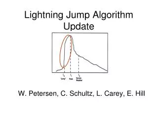
Early Studies • Goodman et al. (1988) demonstrated that total lightning peaked prior to the onset of a microburst. • Williams et al. (1989) showed that the peak total flash rate correlated with the maximum vertical extent of pulse thunderstorms, and preceded maximum outflow velocity by several minutes. • MacGorman et al. (1989) showed that the total flash rate peaked 5 minutes prior to a tornado touchdown, while the cloud-to-ground (CG) flash rate peaked 15 minutes after the peak in intra cloud flash rate. Adapted from Goodman et al. (1988) Adapted from MacGorman et al. (1989)
Previous work:lightning jumps • Williams et al. (1999) examined a large number of severe storms in Central FL • Noticed that the total flash rate “jumped” prior to the onset of severe weather. • Williams also proposed 60 flashes min-1 or greater for separation between severe and non-severe thunderstorms. Adapted from Williams et al. (1999) (above)
The Lightning Jump Framework • Gatlin and Goodman (2010) , JTECH; developed the first lightning jump algorithm • Study proved that it was indeed possible to develop an operational algorithm for severe weather detection • Mainly studied severe thunderstorms • Only 1 non severe storm in a sample of 26 storms Adapted from Gatlin and Goodman (2010)
Schultz et al. (2009), JAMC Thunderstorm breakdown: North Alabama – 83 storms Washington D.C. – 2 storms Houston TX – 13 storms Dallas – 9 storms • Six separate lightning jump configurations tested • Case study expansion: • 107 T-storms analyzed • 38 severe • 69 non-severe • The “2σ” configuration yielded best results • POD beats NWS performance statistics (80-90%); • FAR even better i.e.,15% lower (Barnes et al. 2007) • Caveat: Large difference in sample sizes, more cases are needed to finalize result. • Demonstrated that an operational algorithm is indeed possible.
Schultz et al. 2011, WAF • Expanded to 711 thunderstorms • 255 severe, 456 non severe • Primarily from N. Alabama (555) • Also included • Washington D.C. (109) • Oklahoma (25) • STEPS (22) • Confirmed that total lightning trends perform better than cloud-to-ground (CG) lightning trends for thunderstorm monitoring.
Understanding Limitations Nearly 40% of misses in Schultz et al. (2011) came from low topped supercells, TC rainband storms, and cold season events - Lack of lightning activity inhibited the performance of the algorithm Time-height plot of reflectivity (top) and total flash rate (bot) for an EF-1 producing tornadic storm on March 25, 2010. Tornado touchdown time ~2240 UTC.
NCAR ASP Fellowship and R3 Lightning Jump – Summer 2011 • TITAN work helps put the LJ into the context of an automatic tracker that can be traced to prior LJ work (Schultz et al. 2009, 2011). • Algorithm itself might need to be adjusted to accommodate objective tracking (i.e., no manual corrections). • Use GLM resolution LMA flash data and products (e.g., flash extent density). • Explore limitations and improvements to LJ algorithm with automatic tracking and GLM resolution.
Storm Tracking • Recent work using TITAN at NCAR • Radar radar reflectivity • 35 dBZ, –15 °C • 50 dBZ, 0 °C • Lightning • 1 km Flash Extent Density • 8 km Flash Extent Density, Flash Density • Each of these entities has been tested on multiple flash density/flash extent density thresholds • Goal was to explore lightning tracking methods and get an apples to apples comparison with past studies
A Brief Look at Radar Methods • Following the Schultz et al. methodology (35 dBZ -15°C) and not touching the tracks we obtain the following from TITAN in a period between February and June: • These are only the “isolated” storms within the larger storm sample • Vast majority of this sample is non-severe
Starting Simple:1 km Flash Extent Density • Using 1 km resolution from past studies (e.g., Patrick and Demetriades 2005, McKinney et al. 2008) • Feedback from NWS forecasters was positive toward this • method because it produced more “cellular” features • 3x3 boxcar smoothing applied (mean value) to create a • consolidated feature that is trackable. • Statistics below represent “isolated” storms identified by TITAN.
April 27, 2011 example Midday QLCS tornadic storm Right, time history plot of the lightning trend associated with the storm circled below in the 1 km FED image Left, 1 km FED product. Red circle represents portion of the QLCS that was most active at this time.
Comparison Between Methods 1 km FED Method 35 dbz -15°C Lightning’s limitations: Missing the developmental phase of the storm; impacts lead time (toward edge of LMA in this case) lightning centers can be split (not shown) lightning areas are much smaller as compared to radar
Limitations Tornadic MCV 27 April 2011 Animation courtesy NWS Huntsville No matter how hard we try severe events will be missed due to a lack of lightning
LMA System IssuesMay 26, 2011, 0356-0554 UTC Number of stations contributing to the flash extent density can cause a “blooming” effect which would affect the FED thresholds used to track storms.
GLM Resolution and Proxy We will not have the capability to monitor lightning at 1 km using GLM First step: Must test LMA flash data at 8 km – GLM Resolution Goal: In addition to resolution, must also account for the different measurement of lightning (VHF vs optical) – GLM Proxy
At GLM Resolution By moving to a GLM resolution, we lost individual convective areas within a line. Individual tornadic cells within a line Midday tornadic QLCS, 27 April, 2011
Thresholds tested GLM Resolution Tracking Sensitivity testing on FED and FD products Testing of spatial criteria for track continuation Storm Report numbers Automated verification
Summary of GLM Resolution Tracking • Main failure is in tracking of features • Feature identification numbers changing constantly • Shape and size primary culprits • Affect verification statistics when looking at LJ • Current 2σ should likely not be used alone in real-time operations • Combination of algorithms likely the best candidate • Need to track on a multivariate field…
Trends Still Present 35 Source 10 Source Hailstorm, March 30, 2011 Upward tick in lightning seen about 10 minutes prior to hail, but magnitude of jump not as great
Many Things to Compare… • Validation of a lightning tracking method using the lightning jump will be challenging • Algorithm verification changes drastically with utilization of each algorithm type (2σ, threshold, combination). • Not an apples to apples comparison between tracking methods (FED vs FD, lightning vs radar). • Combination of data types in tracking might be the most useful.
Recent Lessons Learned • Tracking – It’s (almost) all in the tracking now. • Cell tracking is essential but also a limiting factor to LJ performance: dropped tracks, splits/mergers etc. Needs more work. • Tracking on lightning alone likely reduces 2 lead time for some storms – favors multi-sensor approach and will require modifications to LJ algorithm • GLM Resolution • As expected, 8 km LMA lightning resolution can sometimes change/complicate cell identification and tracking • However, lightning trends (and jump) are typically still in GLM resolution cells • GLM resolution and proxy (next) will likely require some adjustments to the lightning jump algorithm and tracking (e.g., threshold choices) • Lightning Jump Algorithm • Since tracking limitations were manually corrected, Schultz et al. studies represent the benchmark (i.e., upside) for what we can expect for verification • Due to automatic tracking limitations, the 2σ method alone will likely not suffice in operations. • To adjust to automated tracking, need to incorporate additional methods that do not require as much cell history (e.g., “Threshold approach” in Schultz et al. 2009)
GLM Proxy Tracking: Challenges GLM Proxy 5-minute Flash Count WDSS-II (wsegmotionII/k-means) cells
GLM Proxy Tracking: Challenges • Colors indicate different cell identifications. • Some of the spikes in GLM proxy flash rate are due to cell mergers. • Time series that end abruptly at high flash rates are due to dropped associations (i.e., from one time step to another, the cell gets a new name and starts a new time series). • When the color changes frequently for one true cell, its time history is compromise. • See Cecil et al. GLM STM poster on “Cell Identification and Tracking for Geostationary Lightning Mapper” for more details and future directions for improvement.
New Start R3 Plans for Year 1:“The GOES-R GLM Lightning Jump Algorithm: Research to Operational Algorithm” • Modify current WDSS-II/K-means cell tracking algorithm and reduce tracking ambiguity • Other GLM fields (GLM flash [or group or event] extent density). Multi-sensor, multi-variable tracking optimization • See Dan Cecil’s GLM STM poster. • Adaptation of LJA for full use of a “Level II” GLM optical flash proxy (e.g., thresholds) • Integration of LJA with ongoing K-means cell tracking on GLM resolution and proxy (acceleration) • Threshold and 2 combined • Participation in National Lightning Jump Field Test coordinated by NOAA NWS (acceleration of PG) • Objective environmental definition of cool season conditions and modification of LJA to improve performance (temporary de-prioritization)
National Lightning Jump Field Demonstration • Guidance Statement • “The Lightning Jump Test (LJT) Project shall run an automated version of the 2σ algorithm using Total Lightning Data (in particular, LMA data) in order to evaluate its performance and effect on watch/warning operations via severe weather verification, with an eye to the future application of the GLM on GOES-R.”
National Lightning Jump Field Demonstration: Goals Establish a fully automated processing method using the “2σ” (2-sigma) algorithm. This includes automated (but not real-time) verification in order to calculate and evaluate POD/FAR/CSI for severe weather forecasts. This is expected to produce a large data set, which can be used for various other post-processing elements, yet to be determined. The results of this test are intended to inform the utility of the GLM data from GOES-R.
National Lightning Jump Field Demonstration • Project Managers: Lead: Tom Filiaggi (NOAA NWS), Steve Goodman (NOAA NESDIS) • Participant Organizations: NASA MSFC, NOAA NESDIS, NOAA NSSL, NOAA NWS (OST-MDL, OST-SPB, WFO’s – MLB, HUN, LWX, LUB), NOAA SPC, TTU, UAHuntsville, U of Maryland, U of Oklahoma • 24 participating individuals (so far) • Area Leads • Algorithms (Carey): Lightning Jump Algorithm (Carey, Schultz), Tracking (Kuhlman), Flash identification (Carey), Lightning Data/Geographic Domain (Stano) • Test Plan (Stumpf) • Data Management (Kuhlman) • Verification (Carey)
National Lightning Jump Field Demonstration: Approximate timeline • Phase 1, Preparation: August 2011 – February 2012 • Identify and tune tracker, LMA flash identification algorithm, lightning jump algorithm • K-means on radar reflectivity at -10C • LMA flash ID algorithm: NSSL/OU/Lak’s code • Will recommend that 2 be updated to 2/threshold blend • Define verification data and methods • Enhanced verification beyond Storm Data (SHAVE - Severe Hazards Analysis and Verification Experiment) • Prepare hardware and define data management plan • Flesh out test plan • Stress test (on archived case data)
National Lightning Jump Field Demonstration: Approximate timeline • Phase 2, Maturation (1st test phase): March 2012 – October 2012 • Run Lightning Jump Algorithm continuously for defined domain and archive data • Dynamic test: continue tuning various aspects as we learn, adapt, and improve • Tracking • Verification • Flash ID/proxy definition • Not yet done for “operational forecaster” environment • Preliminary report to NWS in Summer 2012
National Lightning Jump Field Demonstration: Approximate timeline • Phase 3, Re-evaluation : November 2012 – February 2013 • Evaluate Phase 2 for lessons learned • Incorporate new knowledge from R3 and Phase 2 test • Re-tune and improve algorithms • Tracking improvements, multi-sensor tracking (radar, lightning, and/or IR ?) • Verification (e.g., expand to radar ?) • GLM flash proxy improvements (e.g., resolution, VHF-to-optical). Not clear that this will be ready due to strong feedback to tracking. • Incorporate other lightning proxies (e.g., WTLN etc)?
National Lightning Jump Field Demonstration: Approximate timeline • Phase 4, Full Test : March 2013 – August 2013 • Algorithms should be stable (static) during test • Possibly accomplished in an operational forecasting environment • Some training required for forecasters • Phase 5, Wrap Up: July – September 2013 • Evaluation and NWS reporting by end of FY13 • Phase 6 (?), Additional NWS Test Phases? • UAHuntsville LJ R3 plan PG in Optional Year 3 (FY13) • Remaining issues to test operationally (e.g., more realistic GLM proxy, multi-sensor tracking etc)?