Download
1 / 16
160 likes | 235 Views
Examining the Signal. Examine the signal using a very high-speed system, for example, a 50 MHz digital oscilloscope. Setting the Sampling Conditions. In most circumstances, as when using computers, sampling is DIGITAL. For example, consider two different signals.

E N D
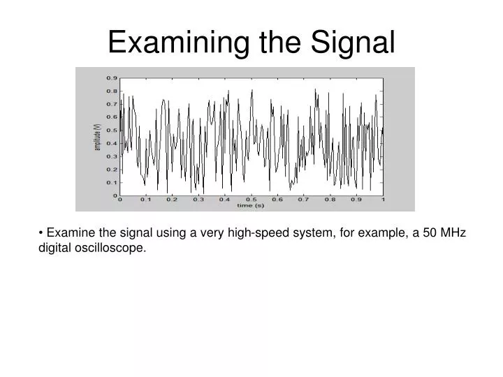
Examining the Signal • Examine the signal using a very high-speed system, for example, a 50 MHz digital oscilloscope.
Setting the Sampling Conditions • In most circumstances, as when using computers, sampling is DIGITAL.
For example, consider two different signals Solid: ‘normal’ (random) population with mean =3 and standard deviation = 0.5 Dotted: same as solid but with 0.001/s additional amplitude decrease The Number of Samples • The number of required samples depends upon what information is needed • → there is not one specific formula for N..
Figure 12.1 Digital Sampling • The analog signal, y(t), is sampled every dt seconds, N times for a period • of T seconds, yielding the digital signal y(rdt), where r = 1, 2, …, N. • For this situation:
Digital Sampling Errors • When is signal is digitally sampled, erroneous results occur if either one • of the following occur:
Digital Sampling Errors • To avoid amplitude ambiguity, set the sample period equal to the least • common (integer) multiple of all of the signal’s contributory periods. The least common multiple or lowest common multiple or smallest common multiple of two integersa and b is the smallest positive integer that is a multiple of both a and b. Since it is a multiple, a and bdivide it without remainder. For example, the least common multiple of the numbers 4 and 6 is 12. (Ref: Wikipedia)
Illustration of Correct Sampling y(t) = 5sin(2pt) → f = 1 Hz with fs = 8 Hz Figure 12.7
Illustration of Aliasing y(t) = sin(20pt) >> f = 10 Hz with fs = 12 Hz
Figures 12.8 and 12.9 The Folding Diagram To determine the aliased frequency, fa: Example: f = 10 Hz; fs = 12 Hz
Aliasing of sin(20pt) y(t) = sin(20pt) → f = 10 Hz with fs = 12 Hz
Aliasing of sin(20pt) y(t) = 5sin(2pt) → f = 1 Hz fs = 1.33 Hz Figure 12.13
In-Class Example • At what cyclic frequency will y(t) = 3sin(4pt) appear if fs = 6 Hz? fs = 4 Hz ? fs = 2 Hz ? fs = 1.5 Hz ?
Correct Sample Time Period y(t) = 3.61sin(4pt+0.59) + 5sin(8pt) Figure 12.16
Sampling with Aliasing y(t) = 5sin(2pt) → f = 1 Hz fs = 1.33 Hz Figure 12.13
Sampling with Amplitude Ambiguity y(t) = 5sin(2pt) → f = 1 Hz fs = 3.33 Hz Figure 12.12
y(t) = 6 + 2sin(pt/2) + 3cos(pt/5) +4sin(pt/5 + p) – 7sin(pt/12) In-Class Example fi (Hz): Ti (s): Smallest sample period that contains all integer multiples of the Ti’s: Smallest sampling to avoid aliasing (Hz):