Download

1 / 41
410 likes | 428 Views
Today’s puzzle. How far can you reach with a stack of n blocks, each 2 units long?. d ( n ). Today’s puzzle. 1. 1/2. 1/3. 1/4. 1/5. 1/6. How far can you reach with a stack of n blocks, each 2 units long? d ( n ) = 1+ 1/2 + 1/3 + 1/4 + 1/5 + 1/6 ….

E N D
Today’s puzzle • How far can you reach with a stack of n blocks, each 2 units long? d(n) Comp 122
Today’s puzzle 1 1/2 1/3 1/4 1/5 1/6 • How far can you reach with a stack of n blocks, each 2 units long? d(n) = 1+ 1/2 + 1/3 + 1/4 + 1/5 + 1/6 … nthharmonic number, Hn =Q(lg n) d(n) Comp 122
Quicksort - Randomized Comp 122, Spring 2004
Quicksort: review Partition(A, p, r) x, i := A[r], p – 1; for j := p to r – 1 do if A[j] x then i := i + 1; A[i] A[j] fi od; A[i + 1] A[r]; return i + 1 Quicksort(A, p, r) if p < r then q := Partition(A, p, r); Quicksort(A, p, q – 1); Quicksort(A, q + 1, r) fi A[p..r] 5 A[p..q – 1] A[q+1..r] Partition 5 5 5 Comp 122
Worst-case Partition Analysis Recursion tree for worst-case partition Split off a single element at each level: T(n) = T(n – 1) + T(0) + PartitionTime(n) = T(n – 1) + (n) = k=1 to n(k) = (k=1 to nk ) = (n2) n n – 1 n – 2 n n – 3 2 1 Comp 122
Best-case Partitioning cn cn/2 cn/2 lg n cn/4 cn/4 cn/4 cn/4 c c c c c c • Each subproblem size n/2. • Recurrence for running time • T(n) 2T(n/2) + PartitionTime(n) = 2T(n/2) + (n) • T(n) = (n lg n) Comp 122
Variations • Quicksort is not very efficient on small lists. • This is a problem because Quicksort will be called on lots of small lists. • Fix 1: Use Insertion Sort on small problems. • Fix 2: Leave small problems unsorted. Fix with one final Insertion Sort at end. • Note: Insertion Sort is very fast on almost-sorted lists. Comp 122
Unbalanced Partition Analysis • What happens if we get poorly-balanced partitions, e.g., something like: T(n) T(9n/10) + T(n/10) + (n)? • Still get (n lg n)!!(As long as the split is of constant proportionality.) • Intuition: Can divide n by c > 1 only (lg n) times before getting 1. • n • • n/c • • n/c2 • • • • 1= n/clogcn n n Roughly logc n levels; Cost per level is O(n). n (Remember: Different base logs are related by a constant.) Comp 122
Intuition for the Average Case • Partitioning is unlikely to happen in the same way at every level. • Split ratio is different for different levels. (Contrary to our assumption in the previous slide.) • Partition produces a mix of “good” and “bad” splits, distributed randomly in the recursion tree. • What is the running time likely to be in such a case? Comp 122
Intuition for the Average Case n Bad split followed by a good split: Produces subarrays of sizes 0, (n – 1)/2 – 1, and (n – 1)/2. Cost of partitioning : (n) + (n-1) = (n). (n) 0 n – 1 (n – 1)/2 (n – 1)/2 – 1 Good split at the first level: Produces two subarrays of size (n – 1)/2. Cost of partitioning : (n). (n) n (n – 1)/2 (n – 1)/2 Situation at the end of case 1 is not worse than that at the end of case 2. When splits alternate between good and bad, the cost of bad split can be absorbed into the cost of good split. Thus, running time is O(n lg n), though with larger hidden constants. Comp 122
Randomized Quicksort • Want to make running time independent of input ordering. • How can we do that? • Make the algorithm randomized. • Make every possible input equally likely. • Can randomly shuffle to permute the entire array. • For quicksort, it is sufficient if we can ensure that every element is equally likely to be the pivot. • So, we choose an element in A[p..r] and exchange it with A[r]. • Because the pivot is randomly chosen, we expect the partitioning to be well balanced on average. Comp 122
Variations (Continued) • Input distribution may not be uniformly random. • Fix 1:Use “randomly” selected pivot. • We’ll analyze this in detail. • Fix 2:Median-of-three Quicksort. • Use median of three fixed elements (say, the first, middle, and last) as the pivot. • To get O(n2) behavior, we must continually be unlucky to see that two out of the three elements examined are among the largest or smallest of their sets. Comp 122
Randomized Version Want to make running time independent of input ordering. Randomized-Quicksort(A, p, r) if p < r then q := Randomized-Partition(A, p, r); Randomized-Quicksort(A, p, q – 1); Randomized-Quicksort(A, q + 1, r) fi Randomized-Partition(A, p, r) i := Random(p, r); A[r] A[i]; Partition(A, p, r) Comp 122
Probabilistic Analysis and Randomized Algorithms Comp 122, Spring 2004
The Hiring Problem • You are using an employment agency to hire a new assistant. • The agency sends you one candidate each day. • You interview the candidate and must immediately decide whether or not to hire that person. But if you hire, you must also fire your current office assistant—even if it’s someone you have recently hired. • Cost to interview is ci per candidate. • Cost to hire isch per candidate. • You want to have, at all times, the best candidate seen so far. • When you interview a candidate who is better than your current assistant, you fire the current assistant and hire the candidate. • You will always hire the first candidate that you interview. • Problem:What is the cost of this strategy? Comp 122
Pseudo-code to Model the Scenario Hire-Assistant (n) best 0 ;;Candidate 0 is a least qualified sentinel candidate for i 1 to n do interview candidate i ifcandidate i is better than candidate best thenbest i hire candidate i • Cost Model: Slightly different from the model considered so far. • However, analytical techniques are the same. • Want to determine the total cost of hiring the best candidate. • If n candidates interviewed and m hired, then cost is nci+mch. • Have to pay nci to interview, no matter how many we hire. • So, focus on analyzing the hiring cost mch. • m varies with order of candidates. Comp 122
Worst-case Analysis • In the worst case, we hire all n candidates. • This happens if each candidate is better than all those who came before. Candidates come in increasing order of quality. • Cost is nci+nch. • If this happens, we fire the agency. What should happen in the typical or average case? Comp 122
Probabilistic Analysis • We need a probability distribution of inputs to determine average-case behavior over all possible inputs. • For the hiring problem, we can assume that candidates come in random order. • Assign a rank rank(i), a unique integer in the range 1 to n to each candidate. • The ordered list rank(1), rank(2), …, rank(n) is a permutation of the candidate numbers 1, 2, …, n. • Let’s assume that the list of ranks is equally likely to be any one of the n! permutations. • The ranks form a uniform random permutation. • Determine the number of candidates hired on an average, assuming the ranks form a uniform random permutation. Comp 122
Randomized Algorithm • Impose a distribution on the inputs by using randomization within the algorithm. • Used when input distribution is not known, or cannot be modeled computationally. • For the hiring problem: • We are unsure if the candidates are coming in a random order. • To make sure that we see the candidates in a random order, we make the following change. • The agency sends us a list of n candidates in advance. • Each day, we randomly choose a candidate to interview. • Thus, instead of relying on the candidates being presented in a random order, we enforce it. Comp 122
Discrete Probability See Appendix C & Chapter 5. Comp 122, Spring 2004
Discrete probability = counting • The language of probability helps count all possible outcomes. • Definitions: • Random Experiment (or Process) • Result (outcome) is not fixed. Multiple outcomes are possible. • Ex: Throwing a fair die. • Sample Space S • Set of all possible outcomes of a random experiment. • Ex: {1, 2, 3, 4, 5, 6} when a die is thrown. • Elementary Event • A possible outcome, element of S, x S; • Ex: 2 – Throw of fair die resulting in 2. • Event E • Subset of S, ES; • Ex: Throw of die resulting in {x> 3} = {4, 5, 6} • Certain event : S • Null event: • Mutual Exclusion • Events A and B are mutually exclusive if AB= . Comp 122
Axioms of Probability & Conclusions • A probability distribution Pr{} on a sample space S is a mapping from events of S to real numbers such that the following are satisfied: • Pr{A} 0 for any event A. • Pr{S} = 1. (Certain event) • For any two mutually exclusive events A and B, Pr(AB ) = Pr(A)+Pr(B). • Conclusions from these axioms: • Pr{} = 0. • If A B, then Pr{A} Pr{B}. • Pr(AB ) = Pr(A)+Pr(B)-Pr(AB) Pr(A)+Pr(B) Comp 122
Independent Events • Events A and B are independent if Pr{A|B} = Pr{A}, if Pr{B} != 0 i.e., if Pr{AB} = Pr{A}Pr{B} • Example: Experiment: Rolling two independent dice. Event A: Die 1 < 3 Event B: Die 2 > 3 A and B are independent. Comp 122
Discrete Random Variables • A random variable X is a function from a sample space S to the real numbers. • If the space is finite or countably infinite, a random variable X is called a discrete random variable. • Maps each possible outcome of an experiment to a real number. • For a random variable X and a real number x, the event X=x is {sS : X(s)=x}. • Pr{X=x} = {sS:X{s}=x}Pr{s} • f(x) = Pr{X=x} is the probability density function of the random variable X. Comp 122
Discrete Random Variables • Example: • Rolling 2 dice. • X: Sum of the values on the two dice. • Pr{X=7} = Pr{(1,6),(2,5),(3,4),(4,3),(5,2),(6,1)} = 6/36 = 1/6. Comp 122
Expectation • Average or mean • The expected value of a discrete random variable X is E[X] = x x Pr{X=x} • Linearity of Expectation • E[X+Y] = E[X]+E[Y], for all X, Y • E[aX+Y]=aE[X]+E[Y], for constant a and all X, Y • For mutually independent random variablesX1, X2, …, Xn • E[X1X2 … Xn] = E[X1]E[X2]…E[Xn] Comp 122
Expectation – Example • Let X be the RV denoting the value obtained when a fair die is thrown. What will be the mean of X, when the die is thrown n times. • Let X1, X2, …, Xn denote the values obtained during the n throws. • The mean of the values is (X1+X2+…+Xn)/n. • Since the probability of getting values 1 thru 6 is (1/6), on an average we can expect each of the 6 values to show up (1/6)n times. • So, the numerator in the expression for mean can be written as (1/6)n·1+(1/6)n·2+…+(1/6)n·6 • The mean, hence, reduces to (1/6)·1+(1/6)·2+…(1/6)·6, whichis what we get if we apply the definition of expectation. Comp 122
Indicator Random Variables • A simple yet powerful technique for computing the expected value of a random variable. • Convenient method for converting between probabilities and expectations. • Helpful in situations in which there may be dependence. • Takes only 2 values, 1 and 0. • Indicator Random Variable for anevent Aof a sample space is defined as: Comp 122
Indicator Random Variable Lemma 5.1 Given a sample space S and an event A in the sample space S, let XA= I{A}. Then E[XA] = Pr{A}. Proof: Let Ā = S – A (Complement of A) Then, E[XA] = E[I{A}] = 1·Pr{A} + 0·Pr{Ā} = Pr{A} Comp 122
Indicator RV – Example Problem: Determine the expected number of heads in n coin flips. Method 1: Without indicator random variables. Let X be the random variable for the number of heads in n flips. Then, E[X] = k=0..nk·Pr{X=k} We solved this last class with a lot of math. Comp 122
Indicator RV – Example • Method 2 : Use Indicator Random Variables • Define n indicator random variables, Xi, 1 i n. • Let Xibe the indicator random variable for the event that the ith flip results in a Head. • Xi = I{the ith flip results in H} • Then X = X1 + X2 + …+ Xn = i=1..nXi. • By Lemma 5.1, E[Xi] = Pr{H} = ½, 1 i n. • Expected number of heads is E[X] = E[i=1..nXi]. • By linearity of expectation, E[i=1..nXi] = i=1..nE[Xi]. • E[X] = i=1..nE[Xi] = i=1..n½ = n/2. Comp 122
Randomized Hire-Assistant Randomized-Hire-Assistant (n) Randomly permute the list of candidates best 0 ;;Candidate 0 is a least qualified dummy candidate for i 1 to n do interview candidate i ifcandidate i is better than candidate best thenbest i hire candidate i How many times do you find a new maximum? Comp 122
Analysis of the Hiring Problem (Probabilistic analysis of the deterministic algorithm) • X – RV that denotes the number of times we hire a new office assistant. • Define indicator RV’s X1, X2, …, Xn. • Xi = I{candidate i is hired}. • As in the previous example, • X = X1 + X2 + …+ Xn • Need to compute Pr{candidate i is hired}. • Pr{candidate i is hired} • i is hired only if i is better than 1, 2,…,i-1. • By assumption, candidates arrive in random order • Candidates 1, 2, …, i arrive in random order. • Each of the i candidates has an equal chance of being the best so far. • Pr{candidate i is the best so far} = 1/i. • E[Xi] = 1/i. (By Lemma 5.1) Comp 122
Analysis of the Hiring Problem • Compute E[X], the number of candidates we expect to hire. By Equation (A.7) of the sum of a harmonic series. Expected hiring cost = O(chln n). Comp 122
Analysis of the randomized hiring problem • Permutation of the input array results in a situation that is identical to that of the deterministic version. • Hence, the same analysis applies. • Expected hiring cost is hence O(chln n). Comp 122
Quicksort - Randomized Comp 122, Spring 2004
Avg. Case Analysisof Randomized Quicksort • Let RV X = number of comparisons over all calls to Partition. • Suffices to compute E[X]. Why? • Notation: • Let z1, z2, …, zn denote the list items (in sorted order). • Let Zij = {zi, zi+1, …, zj}. • Let RV Xij= • Thus, Xij is an indicator random variable. Xij=I{zi is compzred to zj}. 1 if zi is compared to zj 0 otherwise Comp 122
Analysis (Continued) We have: Note: E[Xij] = 0·P[Xij=0] + 1·P[Xij=1] = P[Xij=1] This is a nice property of indicator RVs. (Refer to notes on Probabilistic Analysis.) So, all we need to do is to compute P[zi is compared to zj]. Comp 122
Analysis (Continued) zi and zj are compared iff the first element to be chosen as a pivot from Zij is either zi or zj. Exercise: Prove this. So, Comp 122
Analysis (Continued) Substitute k = j – i. Comp 122
Deterministic vs. Randomized Algorithms Algorithms Deterministic Randomized Worst-case Analysis Probabilistic Analysis Probabilistic Analysis Worst-case Running Time Average Running Time Average Running Time • Deterministic Algorithm : Identical behavior for different runs for a given input. • Randomized Algorithm : Behavior is generally different for different runs for a given input. Comp 122