Download
1 / 30
300 likes | 493 Views
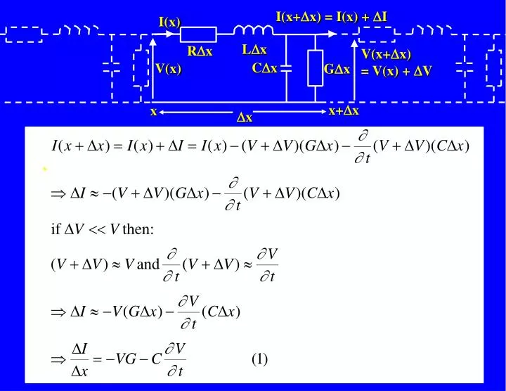
I(x+ D x) = I(x) + D I. I(x). L D x. R D x. V(x+ D x) = V(x) + D V. C D x. V(x). G D x. x+ D x. x. D x. Hence:. Letting Δ x tend to zero:.

E N D
I(x+Dx) = I(x) + DI I(x) LDx RDx V(x+Dx) = V(x) + DV CDx V(x) GDx x+Dx x Dx
Hence: LettingΔx tend to zero: Equations 3 & 4 are called the "Telegrapher's Equations"and are important because they govern the variation of I and V as a function of distance along the line (x) and time (t).
But we can substitute for I/t from one of the Telegrapher's Equations [Equation (4)]: Rearranging: Using similar steps it can also be shown that: The above two equations govern the voltage and current along a general transmission line.
Note the similarity between these two equations and . . . . . . the wave equations obtained from Maxwell's Equations in Prof. Murray's section: Consider the special case of a lossless transmission line, i.e. one for which R = 0 and G = 0. The previous equations reduce to: Equations 9 and 10 describe voltage and current WAVES travelling down the transmission line.
Any function, F, which has t+x/v or t-x/v as the variable is a solution to these equations, v being a constant with the dimensions of velocity (i.e. units of m/s): Solution to the wave equations for a lossless transmission line. Note that F is a function of x AND t. It is not surprising that F can be any function since we can propagate sine waves, square waves, triangular waves and waves of arbitrary shape down e.g. a coaxial cable.
To verify that F(tx/v) is a solution we need to put F into the wave equation and check that If we do that for F(t-x/v), we find: Therefore F(t-x/v) is a solution of the wave equations for the lossless transmission line (Equations 9 and 10) if 1/v2 = LC (or v = 1/√LC) Similarly you can show that F(t+x/v) is a solution if 1/v2 = LC (or v = 1/√LC)
F(t-x/v) F(t+x/v) The “-” and “+” signs in the variable show which direction the wave is moving in. “-” indicates the wave is moving to the right (+ve x direction) “+” indicates the wave is moving to the left (-ve x direction)
Recalling that the velocity of a wave, v, is given by v = fl, then f/v = 1/l. Hence: Putting w = 2p f and b = 2p / l (where b is termed the PHASE CONSTANT): V(x,t) = V1cos[wt - bx] b is termed the phase constant because bx gives the phase of the wave at the point x.
SYLLABUS Part 1 - Introduction and Basics Lecture Topics 1. General definition Practical definition Types of transmission line: TE, TM, TEM modes TEM wave equation - equivalent circuit approach 2. The "Telegrapher's Equations" Solution for lossless transmission lines: F(t±x/v) Simplest case of F(t±x/v) 3. Direction of travel of cos/sin (ωt ±x) waves Phase velocity of a wave on a transmission line General transmission line: attenuation
2.3 Properties of a wave on a transmission line. A wave of frequency 4.5 MHz and phase constant 0.123 rad/m propagates down a lossless transmission line of length 500 m and with μr=1. Find: (i) the wavelength (ii) the velocity of the wave (iii) the phase difference between the phasor voltages at the two ends of the line (iv) the time required for a reference point on the wave to travel down the line (v) the relative permittivity of the dielectric in the line
Direction of travel of cos/sin(wt +bx) waves This figure shows how the function V=V1 sin (wt + bx) changes with time: a point, P, of constant phase moves to the LEFT with time. P l V V1 0 -V1 T = period t = 0 (a) t=T/4 (b) t= T/2 (c) p 2p 3p 4p bx P V V1 0 -V1 p 2p 3p 4p bx P V V1 0 -V1 p 2p 3p 4p bx V=V1 sin (wt + bx)
Direction of travel of cos/sin(wt +bx) waves This figure shows how the function V=V1 sin (wt - bx) changes with time: a point, P, of constant constant phase moves to the RIGHT with time. P l V V1 0 -V1 T = period t = 0 (a) t=T/4 (b) t= T/2 (c) p 2p 3p 4p bx P V V1 0 -V1 p 2p 3p 4p bx P V V1 0 -V1 p 2p 3p 4p bx V=V1 sin (wt - bx)
P V x Phase Velocity of a Wave on a Transmission Line V=V1 sin (wt - bx) The PHASE VELOCITY of a wave is defined as the velocity of a point of constant phase. For a point of constant phase, V is constant, hence wt+ bx = constant To find the velocity of this constant phase point we must obtain x/t, so differentiate the above w.r.t time, t: w +b x/t = 0 \ PHASE VELOCITY = x/t = +w/b = + v
For a lossless transmission line with inductance per unit length L and capacitance per unit length C: Example 2.1 shows that the velocity of a TEM wave on a lossless transmission line is the same as that of an EM wave in the dielectric medium of the line.
General Transmission Line [R g 0, G g 0] Until now we have dealt with the simplest type of transmission line, i.e. a lossless line (R=0 and G=0) …what happens if the line isn’t lossless? Δx LDx RDx CDx GDx
For a lossless line (R = 0 and G = 0) we know that the voltage is governed by the wave equation with solution V = V1e jwt e jx Lossless Line (R = 0 and G = 0) General Line (R g 0, G g 0) For a line which isn't lossless we saw that the voltage is governed by Equation 7: By analogy with the solution for the wave equation, for the general line let's take as a trial solution to Equation 7: V = V1e jwt e gx = V1e(jwt+gx) (14) but take γ to be complex rather than imaginary like j.
V = V1 e jwt e jbx Lossless Line ( is real) V = V1 e jwt e gx General Line (g is complex) Here we are assuming that the time variation is as before but the spatial variation is different and as yet unknown since g is unknown. To check that our trial function is a solution we need to put it in Equation 7 and check that L.H.S. = R.H.S.
For RHS: Substituting for V/t and 2V/t2 in 7:
Comparing (16) and (17), we see that for our trial function to be a solution: γ2V = (R + jwL)(G + jwC)V => g2= (R + jwL)(G + jwC) (18) Thus V1 e(jwt+gx)is a solution to Equation 7 if: g = + {(R + jwL)(G + jwC)}1/2 (19)
The + sign again indicates the direction the wave is travelling in: the solution with e-gxcorresponds to a forward travelling wave (+x direction) the solution with e+gxcorresponds to a backward travelling wave (-x direction) The general solution is V = V1 e jwt e -gx +V2 e jwt e +gx where V1 and V2 are independent arbitrary amplitudes which depend on the circumstances.
Physically, this corresponds to two waves moving simultaneously in opposite directions on the transmission line: V = V1 e jwt e -gx +V2 e jwt e +gx − Backward (Reflected) voltage wave −Forward voltagewave -x +x
V = V1 e jwt e jbx Lossless Line ( is real) V = V1 e jwt e gx General Line (g is complex) We need to check that g reduces to j when the line is lossless – so put R = G = 0 in Equation 19: For the lossless case g = + {(R + jwL)(G + jwC)}1/2 (19) g = +(j2w2LC)1/2 = + jw(LC)1/2 = + jw/v [since v = 1/(LC)1/2] = + jb [since w/b = v]
Thus for the lossless case e+gx=e+ jbx i.e. g is purely imaginary (γ = ±j). In general,g is complex and has both real and imaginary parts: g = +{(R+jwL)(G+jwC)}1/2 = +(a + jb) Hence: e+gx = e+(a+jb)x=e+axe+jbx The factor e+ax operates on the amplitude of the wave, decreasing it exponentially. a is termed the ATTENUATION CONSTANT e+ax gives the amplitude attenuation as the wave travels e+jbxgives the phase change over distance x g is termed the PROPAGATION CONSTANT
For a forward travelling wave: V = V1 e jwt e-gx = V1 e-ax e j(wt-bx) amplitude factor phase factor time variation Voltage V1 x
Derive an expression for the phase velocity of a wave on a general transmission line. Example 3.1 - Phase velocity of a wave Voltage V1 P x
Determine approximate expressions for a and b when w is large (i.e. at high frequencies) or when R and G are small. Example 3.2 - High-frequency expressions for the attenuation and phase constants, a and b.
Example 3.3 - Calculation of a and b. For a parallel wire transmission line the primary line constants at 3 kHz are R = 6.74 Ω/km L = 0.00352 H/km G = 0.29x10⁻⁶ S/km C = 0.0087x10⁻⁶ F/km Find the attenuation and phase constants (a and b) and the phase velocity of the line at 3 kHz. Find also the distance at which the wave amplitude has decayed to 0.1 of its initial value.
Summary q Direction of travel of cos/sin(wt+bx) waves the + sign gives the DIRECTION OF TRAVEL for the waves: + indicates the wave is travelling to the left (i.e. in -x direction) - indicates the wave is travelling to the right (i.e. in +x direction) q The PHASE VELOCITY of a wave on a transmission line is defined as the velocity of a point of constant phase. Phase velocity = v = fl = w/b [ = 1/(LC)1/2 for a lossless line]
q Voltage on a general transmission line [R g 0, G g 0] V = V1e(jwt+gx) where g = +{(R+jwL)(G+jwC)}1/2 = +(a + jb) g is termed the PROPAGATION CONSTANT a is termed the ATTENUATION CONSTANT b is the PHASE CONSTANT V = V1e(jwt-gx) = V1e-axe j(wt-bx) GENERAL SOLUTION is: V = V1ejwte-gx + V2ejwte+gx forward reflected wave wave