Download
1 / 12
120 likes | 209 Views
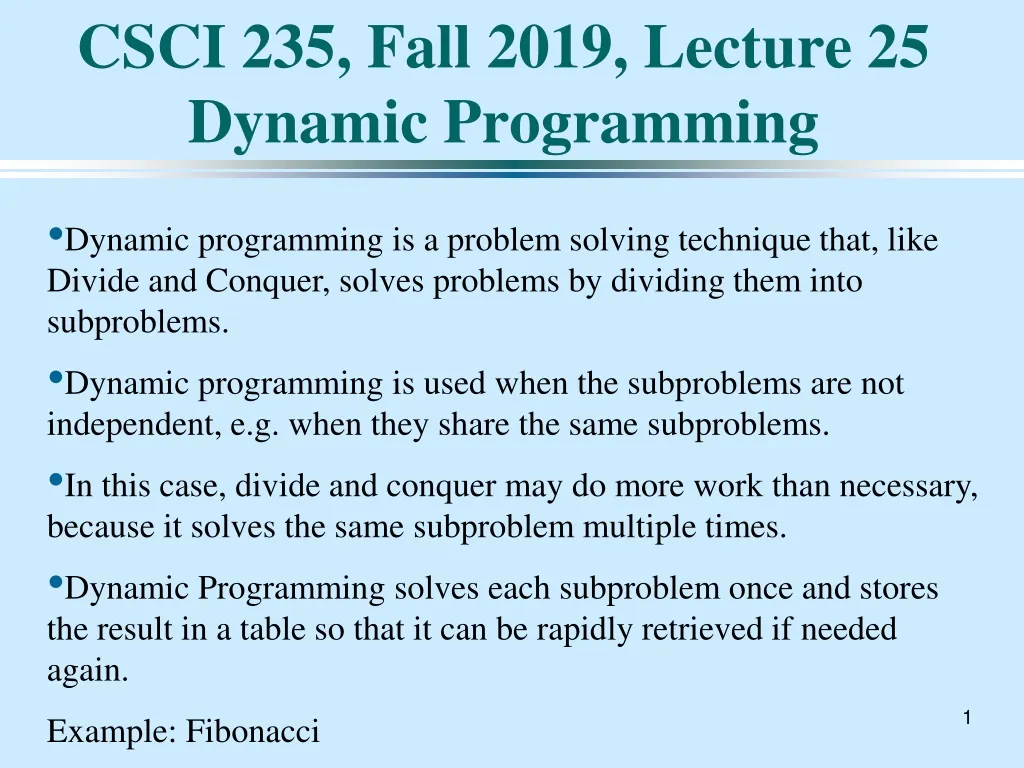
CSCI 235 , Fall 2019, Lecture 25 Dynamic Programming. Dynamic programming is a problem solving technique that, like Divide and Conquer, solves problems by dividing them into subproblems .

E N D
CSCI 235, Fall2019, Lecture 25Dynamic Programming • Dynamic programming is a problem solving technique that, like Divide and Conquer, solves problems by dividing them into subproblems. • Dynamic programming is used when the subproblems are not independent, e.g. when they share the same subproblems. • In this case, divide and conquer may do more work than necessary, because it solves the same subproblem multiple times. • Dynamic Programming solves each subproblem once and stores the result in a table so that it can be rapidly retrieved if needed again. Example: Fibonacci
When do we use Dynamic Programming? • Dynamic programming solves each subproblem once and stores the solution in a table. You can then look up the solution when needed again. • It is often used in Optimization Problems: A problem with many possible solutions for which you want to find an optimal (the best) solution. (There may be more than 1 optimal solution). • Applications: • Control (Cruise control, Robotics, Thermostats) • Flight control (balance factors that oppose one another, e.g. maximize accuracy, minimize time). • Time Sharing: Schedule user and jobs to maximize CPU usage • Other types of scheduling.
Development of Dynamic Programming Algorithm • Characterize the structure of an optimal solution • Recursively define the value of the optimal solution. Like divide and conquer, divide the problem into 2 or more optimal parts recursively. This helps to define what the solution will look like. • Compute the value of the optimal solution from the bottom up (starting with the smallest subproblem). 4. Construct the optimal solution for the entire problem from the computed values of smaller subproblems.
Matrices A Matrix is a rectangular array of quantities: 2x3 Matrix 2x2 Matrix 3x1 Matrix mxn Matrix
Matrix Multiplication To multiply two matrices, multiply the rows in the first matrix by the columns of the second matrix. Example: In general:
Examples a) b)
Matrix Chain Multiplication Problem: Given <A1, A2, A3, ...An> are n matrices, find their product, A1A2A3...An Note that the order of multiplication can yield different running times, even though the result is the same. E.g (A1A2)A3 may have a different running time than A1(A2A3) We will measure running times in terms of the number of scalar multiplications required.
Example We will examine this in class.
The problem Problem: Find the best way to multiply n matrices (where best means the one that uses the minimum number of scalar multiplications). Practical use: Computer Graphics (Long chains of matrices to multiply). Formally: Given <A1, A2, A3, ...An> are n matrices, fully parenthesize the product A1A2A3...An in a way to minimize the number of scalar multiplications.
Examining All Possible Solutions One approach to this problem would be to examine all possible solutions and choose the one that gives the minimum number of multiplications. It can be shown that there are: such solutions. Because of the exponential growth, it would take prohibitive amount of time to do an exhaustive search of all the possibilities.
Number of Scalar Multiplications Multiplying 2 matrices, A1, A2, where A1 is pxq and A2 is qxr takes pqr scalar multiplications. Example: 2x3 3x1 Number of multiplications = 2x3x1 = 6
1. Characterize structure of optimal solution Notation: Ai .. j = AiAi+1Ai+2 . . . Aj An optimal solution of A1 ..n = (A1A2 ...Ak)(Ak+1Ak+2 ...An), 1<=k<n Cost = cost of computing A1 .. k + cost of computing Ak+1 .. n + cost to multiply the 2 results together. For the solution to be optimal, we must first find the optimal solutions to the subproblems: A1 .. k and Ak+1 .. n (Why must they be optimal solutions?) Example: A1A2A3A4