Novel features in this model:

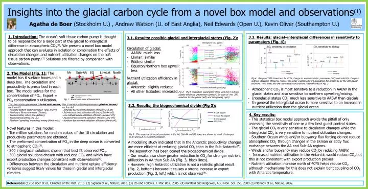
1. Insights into the glacial carbon cycle from a novel box model and observations(1) Agatha de Boer (Stockholm U.) , Andrew Watson (U. of East Anglia), Neil Edwards (Open U.), Kevin Oliver (Southampton U.) 1. Introduction:The ocean’s soft tissue carbon pump is thought to be responsible for a large part of the glacial to interglacial difference in atmospheric CO2(2). We present a novel box model approach that can evaluate in isolation or combination the effects of circulation changes and nutrient utilization changes on the soft tissue carbon pump.(1) Solutions are filtered by comparison with observations. 3.3. Results; glacial–interglacial differences in sensitivity to parameters (Fig. 4): 3.1. Results; possible glacial and interglacial states (Fig. 2): Atmospheric CO2 (ppmv) • Circulation of glacial: • AABW: much less • Ekman: similar • Eddies: similar • Equator/Northern box upwell: less Atm pCO2 AA Sub-AA EQ LowLat North 2. The Model (Fig. 1):The model has 6 surface boxes and a deep box. The circulation and productivity is prescribed in each box. The model solves for the concentration of PO4. Export = PO4 concentration x utilization. • Nutrient utilization efficiency in glacial: • Antarctic: slightly reduced • All other latitudes: increased Fig 4: Range of CO2 drawdown for 15 Sv change in each circulation parameter (left) and a 6e10/s change in nutrient utilization efficiency (right). The range is obtained from calculating the sensitivity for the 300 glacial solutions (solid lines) and the 300 interglacial solutions (dashed lines) in Fig. 2 Preformed Nutrients (µ mol/kg) • Atmospheric CO2 is most sensitive to a reduction in AABW in the glacial states and also sensitive to northern upwelling/mixing. • Interglacial states CO2 much less sensitive to AABW than glacials • In general the interglacial ocean is more sensitive to an increase in nutrient utilization than the glacial ocean. Fig 2: The 5 circulation parameters (top) and the 5 nutrient uptake efficiency parameters (bottom) for each of the 300 solutions for the glacial (left) and interglacial( right). Fig 1: Boxes and their abbreviations. The 5 circulation parameters (circled solid arrows) are from left: - Antarctic Bottom Water formation rate( AABW); - Northward Ekman transport (Ekman); - Southern Eddy return flow (Eddies); - Equatorial Upwelling (Eq Up); - Northern ‘upwelling’ from deep mixing (North mix). The 5 nutrient utilization parameters (dashed arrows) are from left - Antarctic box nutrient utilization efficiency (AA eff) - Sub-Antarctic box utilization efficiency (Sub-AA eff); - Low latitude boxes utilization efficiency (LowLat eff); - Equatorial box nutrient utilization efficiency (EQ eff); - Northern box nutrient utilization efficiency (North eff); 3.2. Results; the biogeochemical divide (Fig 3): • 4. Key results: • - This statistical box model approach avoids the pitfall of only assessing the sensitivity of one or a few best guest control states. • - The glacial CO2 is very sensitive to circulation changes while the interglacial CO2 is very sensitive to nutrient utilization changes. • Southern Ocean winds and/or buoyancy flux forcing do not reduce atmospheric CO2 through changes in the Ekman or Eddy flux exchange between the AA and Sub-AA regions. • - Winds and/or buoyancy may reduce CO2 by reducing AABW. • - Increased nutrient utilization in the Antarctic would reduce CO2 but this is not consistent with export production proxies. • - Nutrient utilization increase north of 40°S helps reduce CO2although mechanisms for this does not explain tight coupling of CO2 with Antarctic temperature. • Novel features in this model: • Ten million solutions for random values of the 10 circulation and productivity parameters are obtained. • The preformed concentration of PO4 in the deep ocean is converted to atmospheric CO2(3). • 300 interglacial solutions chosen that best fit observed PO4. • 300 glacial solutions chosen with reduced CO2 and which have export production changes consistent with observations(4). • - Differences between the circulation and nutrient uptake efficiency variables suggest likely values for these in glacial and interglacial climates. Fig 3: The response of export production in the AA, Sub-AA and EQ boxes are shown as result of changes in AA and Sub-AA nutrient utilization. A modelling study indicated that in the Antarctic productivity changes are more efficient at reducing glacial CO2 than in the Sub-Antarctic(5). The separation has been coined the biogeochemical divide. - Our results also show greater reduction in CO2 for stronger nutrient utilization in AA than Sub-AA (Fig. 3, black lines). - However, high Antarctic utilization is not a realistic glacial result (Fig. 2, bottom) because it causes a strong increase in export production (Fig. 3, left) which is not observed(4). References: (1) De Boer et al., Climates of the Past. 2010. (2) Sigman et al., Nature, 2010. (3) Ito and Follows, J. Mar. Res., 2005. (4) Kohlfeld and Ridgewell, AGU Mon. Ser. 350, 2009.(5) Marinov et al., Nature, 2006.