Summary of MDPs (until Now)

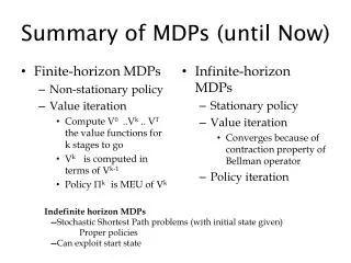
1. Summary of MDPs (until Now) • Finite-horizon MDPs • Non-stationary policy • Value iteration • Compute V0 ..Vk .. VT the value functions for k stages to go • Vk is computed in terms of Vk-1 • Policy Pk is MEU of Vk • Infinite-horizon MDPs • Stationary policy • Value iteration • Converges because of contraction property of Bellman operator • Policy iteration Indefinite horizon MDPs --Stochastic Shortest Path problems (with initial state given) Proper policies --Can exploit start state

2. Use heuristic search (and reachability information) LAO*, RTDP Use execution and/or Simulation “Actual Execution” Reinforcement learning (Main motivation for RL is to “learn” the model) “Simulation” –simulate the given model to sample possible futures Policy rollout, hindsight optimization etc. Use “factored” representations Factored representations for Actions, Reward Functions, Values and Policies Directly manipulating factored representations during the Bellman update Ideas for Efficient Algorithms..

3. VI and PI approaches use Dynamic Programming Update Set the value of a state in terms of the maximum expected value achievable by doing actions from that state. They do the update for every statein the state space Wasteful if we know the initial state(s) that the agent is starting from Heuristic search (e.g. A*/AO*) explores only the part of the state space that is actually reachable from the initial state Even within the reachable space, heuristic search can avoid visiting many of the states. Depending on the quality of the heuristic used.. But what is the heuristic? An admissible heuristic is a lowerbound on the cost to reach goal from any given state It is a lowerbound on J*! Heuristic Search vs. Dynamic Programming (Value/Policy Iteration)

4. Real Time Dynamic Programming[Barto, Bradtke, Singh’95] Trial: simulate greedy policy starting from start state; perform Bellman backup on visited states RTDP: repeat Trials until cost function converges RTDP was originally introduced for Reinforcement Learning For RL, instead of “simulate” you “execute” You also have to do “exploration” in addition to “exploitation”  with probability p, follow the greedy policy with 1-p pick a random action

5. Stochastic Shortest Path MDP 0 0

6. RTDP Trial Min s0 Jn Qn+1(s0,a) agreedy = a2 Jn ? a1 Jn Goal a2 ? Jn+1(s0) Jn a3 ? Jn Jn Jn

7. Greedy “On-Policy” RTDP without execution Using the current utility values, select the action with the highest expected utility (greedy action) at each state, until you reach a terminating state. Update the values along this path. Loop back—until the values stabilize

8. Comments Properties if all states are visited infinitely often then Jn→ J* Only relevant states will be considered A state is relevant if the optimal policy could visit it.  Notice emphasis on “optimal policy”—just because a rough neighborhood surrounds National Mall doesn’t mean that you will need to know what to do in that neighborhood Advantages Anytime: more probable states explored quickly Disadvantages complete convergence is slow! no termination condition Do we care about complete convergence? Think Cpt. Sullenberger

9. Labeled RTDP [Bonet&Geffner’03] Initialise J0 with an admissible heuristic ⇒Jn monotonically increases Label a state as solved if the Jn for that state has converged Backpropagate ‘solved’ labeling Stop trials when they reach any solved state Terminate when s0 is solved Converged means bellman residual is less than e high Q costs s ? G t best action ) J(s) won’t change! high Q costs s G both s and t get solved together

11. Probabilistic Planning --The competition (IPPC) --The Action language.. (PPDDL)

13. Factored Representations: Actions • Actions can be represented directly in terms of their effects on the individual state variables (fluents). The CPTs of the BNs can be represented compactly too! • Write a Bayes Network relating the value of fluents at the state before and after the action • Bayes networks representing fluents at different time points are called “Dynamic Bayes Networks” • We look at 2TBN (2-time-slice dynamic bayes nets) • Go further by using STRIPS assumption • Fluents not affected by the action are not represented explicitly in the model • Called Probabilistic STRIPS Operator (PSO) model

14. Action CLK

17. Not ergodic

20. How to compete? Policy Computation Exec Select ex Select ex Select ex Select ex Off-line policy generation Online action selection Loop Compute the best action for the current state execute it get the new state Pros: Provides fast first response Cons: May paint itself into a corner.. • First compute the whole policy • Get the initial state • Compute the optimal policy given the initial state and the goals • Then just execute the policy • Loop • Do action recommended by the policy • Get the next state • Until reaching goal state • Pros: Can anticipate all problems; • Cons: May take too much time to start executing

21. 1st IPPC & Post-Mortem.. IPPC Competitors Results and Post-mortem To everyone’s surprise, the replanning approach wound up winning the competition. Lots of hand-wringing ensued.. May be we should require that the planners really really use probabilities? May be the domains should somehow be made “probabilistically interesting”? Current understanding: No reason to believe that off-line policy computation must dominate online action selection The “replanning” approach is just a degenerate case of hind-sight optimization • Most IPPC competitors used different approaches for offline policy generation. • One group implemented a simple online “replanning” approach in addition to offline policy generation • Determinize the probabilistic problem • Most-likely vs. All-outcomes • Loop • Get the state S; Call a classical planner (e.g. FF) with [S,G] as the problem • Execute the first action of the plan • Umpteen reasons why such an approach should do quite badly..

22. FF-Replan • Simple replanner • Determinizes the probabilistic problem • Solves for a plan in the determinized problem a3 G a5 a4 a2 a1 a2 a3 a4 S G

23. All Outcome Replanning (FFRA) ICAPS-07 Effect 1 Action1 Effect 1 Probability1 Action Probability2 Effect 2 Action2 Effect 2 27

24. Reducing calls to FF.. • We can reduce calls to FF by memoizing successes • If we were given s0 and sG as the problem, and solved it using our determinization to get the plan s0—a0—s1—a1—s2—a2—s3…an—sG • Then in addition to sending a1 to the simulator, we can memoize {si—ai} as the partial policy. • Whenever a new state is given by the simulator, we can see if it is already in the partial policy • Additionally, FF-replan can consider every state in the partial policy table as a goal state (in that if it reaches them, it knows how to get to goal state..)

25. Hindsight Optimization for Anticipatory Planning/Scheduling • Consider a deterministic planning (scheduling) domain, where the goals arrive probabilistically • Using up resources and/or doing greedy actions may preclude you from exploiting the later opportunities • How do you select actions to perform? • Answer: If you have a distribution of the goal arrival, then • Sample goals upto a certain horizon using this distribution • Now, we have a deterministic planning problem with known goals • Solve it; do the first action from it. • Can improve accuracy with multiple samples • FF-Hop uses this idea for stochastic planning. In anticipatory planning, the uncertainty is exogenous (it is the uncertain arrival of goals). In stochastic planning, the uncertainty is endogenous (the actions have multiple outcomes)

26. Probabilistic Planning(goal-oriented) Left Outcomes are more likely Action Maximize Goal Achievement I Probabilistic Outcome A1 A2 Time 1 A1 A1 A1 A1 A2 A2 A2 A2 Time 2 Dead End Action Goal State State 30

27. Problems of FF-Replan and better alternative sampling FF-Replan’s Static Determinizations don’t respect probabilities. We need “Probabilistic and Dynamic Determinization” Sample Future Outcomes and Determinization in Hindsight Each Future Sample Becomes a Known-Future Deterministic Problem 33

28. Hindsight Optimization(Online Computation of VHS ) • Pick action a with highest Q(s,a,H) where • Q(s,a,H) = R(s,a) + ST(s,a,s’)V*(s’,H-1) • Compute V* by sampling • H-horizon future FH for M = [S,A,T,R] • Mapping of state, action and time (h<H) to a state • S × A × h → S • Common-random number (correlated) vs. independent futures.. • Time-independent vs. Time-dependent futures • Value of a policy π for FH • R(s,FH, π) • V*(s,H) = maxπ EFH [ R(s,FH,π) ] • But this is still too hard to compute.. • Let’s swap max and expectation • VHS(s,H) = EFH [maxπ R(s,FH,π)] • maxπ R(s,FH-1,π) is approximated by FF plan • VHS overestimates V* • Why? • Intuitively, because VHS can assume that it can use different policies in different futures; while V* needs to pick one policy that works best (in expectation) in all futures. • But then, VFFRa overestimates VHS • Viewed in terms of J*, VHS is a more informed admissible heuristic.. 34

29. Implementation FF-Hindsight Constructs a set of futures • Solves the planning problem using the H-horizon futures using FF • Sums the rewards of each of the plans • Chooses action with largest Qhs value

30. Probabilistic Planning(goal-oriented) Left Outcomes are more likely Action Maximize Goal Achievement I Probabilistic Outcome A1 A2 Time 1 A1 A1 A1 A1 A2 A2 A2 A2 Time 2 Dead End Action Goal State State 38

31. Improvement Ideas • Reuse • Generated futures that are still relevant • Scoring for action branches at each step • If expected outcomes occur, keep the plan • Future generation • Not just probabilistic • Somewhat even distribution of the space • Adaptation • Dynamic width and horizon for sampling • Actively detect and avoid unrecoverable failures on top of sampling

32. Hindsight Sample 1 Left Outcomes are more likely Action Maximize Goal Achievement I Probabilistic Outcome A1 A2 Time 1 A1 A1 A1 A1 A2 A2 A2 A2 Time 2 A1: 1 A2: 0 Dead End Action Goal State State 40

33. Exploiting Determinism Plans generated for chosen action, a* S1 S1 S1 Longest prefix for each plan is identified and executed without running ZSL, OSL or FF! a* a* a* G G G

34. Handling unlikely outcomes:All-outcome Determinization • Assign each possible outcome an action • Solve for a plan • Combine the plan with the plans from the HOP solutions

35. Relaxations for Stochastic Planning • Determinizations can also be used as a basis for heuristics to initialize the V for value iteration [mGPT; GOTH etc] • Heuristics come from relaxation • We can relax along two separate dimensions: • Relax –ve interactions • Consider +ve interactions alone using relaxed planning graphs • Relax uncertainty • Consider determinizations • Or a combination of both!

36. Solving Determinizations • If we relax –ve interactions • Then compute relaxed plan • Admissible if optimal relaxed plan is computed • Inadmissible otherwise • If we keep –ve interactions • Then use a deterministic planner (e.g. FF/LPG) • Inadmissible unless the underlying planner is optimal

37. Dimensions of Relaxation 3 4 Negative Interactions Increasing consideration  1 2 Uncertainty Relaxed Plan Heuristic 1 Reducing Uncertainty Bound the number of stochastic outcomes  Stochastic “width” McLUG 2 FF/LPG 3 4 Limited width stochastic planning?

38. Dimensions of Relaxation Uncertainty -ve interactions

39. Expressiveness v. Cost Node Expansions v. Heuristic Computation Cost Limited width stochastic planning FF McLUG Nodes Expanded FF-Replan Computation Cost h = 0 FFR FF

41. Reducing Heuristic Computation Cost by exploiting factored representations • The heuristics computed for a state might give us an idea about the heuristic value of other “similar” states • Similarity is possible to determine in terms of the state structure • Exploit overlapping structure of heuristics for different states • E.g. SAG idea for McLUG • E.g. Triangle tables idea for plans (c.f. Kolobov)

42. A Plan is a Terrible Thing to Waste • Suppose we have a plan • s0—a0—s1—a1—s2—a2—s3…an—sG • We realized that this tells us not just the estimated value of s0, but also of s1,s2…sn • So we don’t need to compute the heuristic for them again • Is that all? • If we have states and actions in factored representation, then we can explain exactly what aspects of si are relevant for the plan’s success. • The “explanation” is a proof of correctness of the plan • Can be based on regression (if the plan is a sequence) or causal proof (if the plan is a partially ordered one. • The explanation will typically be just a subset of the literals making up the state • That means actually, the plan suffix from si may actually be relevant in many more states that are consistent with that explanation

43. Triangle Table Memoization • Use triangle tables / memoization C B A A B C If the above problem is solved, then we don’t need to call FF again for the below: B A A B

44. Explanation-based Generalization (of Successes and Failures) • Suppose we have a plan P that solves a problem [S, G]. • We can first find out what aspects of S does this plan actually depend on • Explain (prove) the correctness of the plan, and see which parts of S actually contribute to this proof • Now you can memoize this plan for just that subset of S

45. Factored Representations: Reward, Value and Policy Functions • Reward functions can be represented in factored form too. Possible representations include • Decision trees (made up of fluents) • ADDs (Algebraic decision diagrams) • Value functions are like reward functions (so they too can be represented similarly) • Bellman update can then be done directly using factored representations..

47. SPUDDs use of ADDs

48. Direct manipulation of ADDs in SPUDD