Download

1 / 57
580 likes | 666 Views
Samples and populations. The normal and standard normal. Sporiš Goran, PhD. http://kif.hr/predmet/mki http://www.science4performance.com/. The Normal Distribution. f(X). Changing μ shifts the distribution left or right. Changing σ increases or decreases the spread. σ. μ. X.

E N D
Samples and populations The normal and standard normal Sporiš Goran, PhD. http://kif.hr/predmet/mki http://www.science4performance.com/
The Normal Distribution f(X) Changingμshifts the distribution left or right. Changing σ increases or decreases the spread. σ μ X
This is a bell shaped curve with different centers and spreads depending on and The Normal Distribution:as mathematical function (pdf) Note constants: =3.14159 e=2.71828
The Normal PDF It’s a probability function, so no matter what the values of and , must integrate to 1!
Normal distribution is defined by its mean and standard dev. E(X)= = Var(X)=2 = Standard Deviation(X)=
**The beauty of the normal curve: No matter what and are, the area between - and + is about 68%; the area between -2 and +2 is about 95%; and the area between -3 and +3 is about 99.7%. Almost all values fall within 3 standard deviations.
68% of the data 95% of the data 99.7% of the data 68-95-99.7 Rule
How good is rule for real data? Check some example data: The mean of the weight of the women = 127.8 The standard deviation (SD) = 15.5
112.3 143.3 68% of 120 = .68x120 = ~ 82 runners In fact, 79 runners fall within 1-SD (15.5 lbs) of the mean. 127.8
96.8 158.8 95% of 120 = .95 x 120 = ~ 114 runners In fact, 115 runners fall within 2-SD’s of the mean. 127.8
81.3 174.3 99.7% of 120 = .997 x 120 = 119.6 runners In fact, all 120 runners fall within 3-SD’s of the mean. 127.8
Example • Suppose SAT scores roughly follows a normal distribution in the U.S. population of college-bound students (with range restricted to 200-800), and the average math SAT is 500 with a standard deviation of 50, then: • 68% of students will have scores between 450 and 550 • 95% will be between 400 and 600 • 99.7% will be between 350 and 650
Example • BUT… • What if you wanted to know the math SAT score corresponding to the 90th percentile (=90% of students are lower)? P(X≤Q) = .90 Solve for Q?….Yikes!
The Standard Normal (Z):“Universal Currency” The formula for the standardized normal probability density function is
The Standard Normal Distribution (Z) All normal distributions can be converted into the standard normal curve by subtracting the mean and dividing by the standard deviation: Somebody calculated all the integrals for the standard normal and put them in a table! So we never have to integrate! Even better, computers now do all the integration.
Comparing X and Z units 100 200 X ( = 100, = 50) 0 2.0 Z ( = 0, = 1)
Example • For example: What’s the probability of getting a math SAT score of 575 or less, =500 and =50? • i.e., A score of 575 is 1.5 standard deviations above the mean Yikes! But to look up Z= 1.5 in standard normal chart (or enter into SAS) no problem! = .9332
Practice problem If birth weights in a population are normally distributed with a mean of 109 oz and a standard deviation of 13 oz, • What is the chance of obtaining a birth weight of 141 oz or heavier when sampling birth records at random? • What is the chance of obtaining a birth weight of 120 or lighter?
Answer • What is the chance of obtaining a birth weight of 141 oz or heavier when sampling birth records at random? From the chart or SAS Z of 2.46 corresponds to a right tail (greater than) area of: P(Z≥2.46) = 1-(.9931)= .0069 or .69 %
Answer b. What is the chance of obtaining a birth weight of 120 or lighter? From the chart or SAS Z of .85 corresponds to a left tail area of: P(Z≤.85) = .8023= 80.23%
Z=1.51 Z=1.51 Looking up probabilities in the standard normal table What is the area to the left of Z=1.51 in a standard normal curve? Area is 93.45%
The “probnorm(Z)” function gives you the probability from negative infinity to Z (here 1.5) in a standard normal curve. The “probit(p)” function gives you the Z-value that corresponds to a left-tail area of p (here .93) from a standard normal curve. The probit function is also known as the inverse standard normal function. Normal probabilities in SAS data _null_; theArea=probnorm(1.5); put theArea; run; 0.9331927987 And if you wanted to go the other direction (i.e., from the area to the Z score (called the so-called “Probit” function data _null_; theZValue=probit(.93); put theZValue; run; 1.4757910282
Probit function: the inverse (area)= Z: gives the Z-value that goes with the probability you want For example, recall SAT math scores example. What’s the score that corresponds to the 90th percentile? In Table, find the Z-value that corresponds to area of .90 Z= 1.28 Or use SAS data _null_; theZValue=probit(.90); put theZValue; run; 1.2815515655 If Z=1.28, convert back to raw SAT score 1.28 = X – 500 =1.28 (50) X=1.28(50) + 500 = 564 (1.28 standard deviations above the mean!) `
Are my data “normal”? • Not all continuous random variables are normally distributed!! • It is important to evaluate how well the data are approximated by a normal distribution
Are my data normally distributed? • Look at the histogram! Does it appear bell shaped? • Compute descriptive summary measures—are mean, median, and mode similar? • Do 2/3 of observations lie within 1 std dev of the mean? Do 95% of observations lie within 2 std dev of the mean? • Look at a normal probability plot—is it approximately linear? • Run tests of normality (such as Kolmogorov-Smirnov). But, be cautious, highly influenced by sample size!
Data from our class… Median = 6 Mean = 7.1 Mode = 0 SD = 6.8 Range = 0 to 24 (= 3.5 σ)
Data from our class… Median = 5 Mean = 5.4 Mode = none SD = 1.8 Range = 2 to 9 (~ 4 σ)
Data from our class… Median = 3 Mean = 3.4 Mode = 3 SD = 2.5 Range = 0 to 12 (~ 5 σ)
Data from our class… Median = 7:00 Mean = 7:04 Mode = 7:00 SD = :55 Range = 5:30 to 9:00 (~4 σ)
13.9 0.3 Data from our class… 7.1 +/- 6.8 = 0.3 – 13.9
Data from our class… 7.1 +/- 2*6.8 = 0 – 20.7
Data from our class… 7.1 +/- 3*6.8 = 0 – 27.5
3.6 7.2 Data from our class… 5.4 +/- 1.8 = 3.6 – 7.2
9.0 1.8 Data from our class… 5.4 +/- 2*1.8 = 1.8 – 9.0
10 0 Data from our class… 5.4 +/- 3*1.8 = 0– 10
0.9 5.9 Data from our class… 3.4 +/- 2.5= 0.9 – 7.9
0 8.4 Data from our class… 3.4 +/- 2*2.5= 0 – 8.4
0 10.9 Data from our class… 3.4 +/- 3*2.5= 0 – 10.9
6:09 7:59 Data from our class… 7:04+/- 0:55 = 6:09 – 7:59
5:14 8:54 Data from our class… 7:04+/- 2*0:55 = 5:14 – 8:54
4:19 9:49 Data from our class… 7:04+/- 2*0:55 = 4:19 – 9:49
The Normal Probability Plot • Normal probability plot • Order the data. • Find corresponding standardized normal quantile values: • Plot the observed data values against normal quantile values. • Evaluate the plot for evidence of linearity.
Normal probability plot coffee… Right-Skewed! (concave up)
Normal probability plot love of writing… Neither right-skewed or left-skewed, but big gap at 6.
Norm prob. plot Exercise… Right-Skewed! (concave up)
Norm prob. plot Wake up time Closest to a straight line…
Formal tests for normality • Results: • Coffee: Strong evidence of non-normality (p<.01) • Writing love: Moderate evidence of non-normality (p=.01) • Exercise: Weak to no evidence of non-normality (p>.10) • Wakeup time: No evidence of non-normality (p>.25)
Normal approximation to the binomial When you have a binomial distribution where n is large and p is middle-of-the road (not too small, not too big, closer to .5), then the binomial starts to look like a normal distribution in fact, this doesn’t even take a particularly large n Recall: What is the probability of being a smoker among a group of cases with lung cancer is .6, what’s the probability that in a group of 8 cases you have less than 2 smokers?
Starting to have a normal shape even with fairly small n. You can imagine that if n got larger, the bars would get thinner and thinner and this would look more and more like a continuous function, with a bell curve shape. Here np=4.8. .27 0 7 1 2 3 4 5 6 8 Normal approximation to the binomial When you have a binomial distribution where n is large and p isn’t too small (rule of thumb: mean>5), then the binomial starts to look like a normal distribution Recall: smoking example…