Download
1 / 76
760 likes | 870 Views
Probabilistic Methods for Interpreting Electron-Density Maps. Frank DiMaio University of Wisconsin – Madison Computer Sciences Department dimaio@cs.wisc.edu. 3D Protein Structure. backbone. backbone sidechain. backbone sidechain C -a l p h a. ALA. LEU. PRO. VAL. ARG. ?. ?. ?.

E N D
Probabilistic Methods for Interpreting Electron-Density Maps Frank DiMaio University of Wisconsin – Madison Computer Sciences Department dimaio@cs.wisc.edu
3D Protein Structure backbone backbone sidechain backbone sidechain C-alpha
ALA LEU PRO VAL ARG ? ? ? 3D Protein Structure … …
High-Throughput Structure Determination • Protein-structure determination important • Understanding function of a protein • Understanding mechanisms • Targets for drug design • Some proteins produce poor density maps • Interpreting poor electron-density maps is very (human) laborious • I aim to automatically interpret poor-quality electron-density maps
… … Electron-Density Map Interpretation GIVEN: 3D electron-density map, (linear) amino-acid sequence
… … Electron-Density Map Interpretation FIND:All-atom Protein Model
Density Map Resolution 1.0Å 2.0Å 3.0Å 4.0Å Ioerger et al. (2002) Terwilliger (2003) Morris et al. (2003) My focus
Thesis Contributions • A probabilistic approach to protein-backbone tracingDiMaio et al., Intelligent Systems for Molecular Biology (2006) • Improved template matching in electron-density mapsDiMaio et al., IEEE Conference on Bioinformatics and Biomedicine (2007) • Creating all-atom protein models using particle filteringDiMaio et al. (under review) • Pictorial structures for atom-level molecular modelingDiMaio et al., Advances in Neural Information Processing Systems (2004) • Improving the efficiency of belief propagationDiMaio and Shavlik, IEEE International Conference on Data Mining (2006) • Iterative phase improvement in ACMI
ACMI Overview • Phase 1: Local pentapeptide search (ISMB 2006, BIBM 2007) • Independent amino-acid search • Templates model 5-mer conformational space • Phase 2: Coarse backbone model(ISMB 2006, ICDM 2006) • Protein structural constraints refine local search • Markov field (MRF) models pairwise constraints • Phase 3: Sample all-atom models • Particle filtering samples high-prob. structures • Probs. from MRF guide particle trajectories
ACMI Overview • Phase 1: Local pentapeptide search (ISMB 2006, BIBM 2007) • Independent amino-acid search • Templates model 5-mer conformational space • Phase 2: Coarse backbone model(ISMB 2006, ICDM 2006) • Protein structural constraints refine local search • Markov field (MRF) models pairwise constraints • Phase 3: Sample all-atom models • Particle filtering samples high-prob. structures • Probs. from MRF guide particle trajectories
5-mer Lookup …SAWCVKFEKPADKNGKTE… • ACMI searches map for each template independently • Spherical-harmonic decomposition allows rapid search of all template rotations Protein DB
Spherical-Harmonic Decomposition f (θ,φ)
map-regionsampled in spherical shells sampled region of density in 5A sphere template-densitysampled in spherical shells calculated (expected) density in 5A sphere 5-mer Fast Rotation Search electron density map pentapeptide fragment from PDB (the “template”)
map-region spherical-harmonic coefficients map-regionsampled in spherical shells correlationcoefficientas functionof rotation template-densitysampled in spherical shells template spherical-harmonic coefficients 5-mer Fast Rotation Search fast-rotation function(Navaza 2006, Risbo 1996)
correlation coefficients over density mapti (ui) probability distribution over density map P(5-mer at ui|EDM) Convert Scores to Probabilities Bayes’ rule scan density map for fragment
ACMI Overview • Phase 1: Local pentapeptide search (ISMB 2006, BIBM 2007) • Independent amino-acid search • Templates model 5-mer conformational space • Phase 2: Coarse backbone model(ISMB 2006, ICDM 2006) • Protein structural constraints refine local search • Markov field (MRF) models pairwise constraints • Phase 3: Sample all-atom models • Particle filtering samples high-prob. structures • Probs. from MRF guide particle trajectories
Probabilistic Backbone Model • Trace assigns a position and orientation ui={xi, qi} to each amino acid i • The probability of a trace U={ui} is • This full joint probability intractable to compute • Approximate using pairwise Markov field
ALA GLY LYS LEU SER Pairwise Markov-Field Model • Joint probabilities defined on a graph as product of vertex and edge potentials
ACMI’s Backbone Model ALA GLY LYS LEU SER Observational potentialstie the map to the model
ALA GLY LYS LEU SER ACMI’s Backbone Model • Adjacency constraints ensure adjacent amino acids are ~3.8Å apart and in proper orientation • Occupancy constraints ensure nonadjacent amino acids do not occupy same 3D space
Backbone Model Potential Constraints between adjacent amino acids × =
Backbone Model Potential Constraints between all other amino acid pairs
Backbone Model Potential Observational (“template-matching”) probabilities
Inferring Backbone Locations • Want to find backbone layout that maximizes
Inferring Backbone Locations • Want to find backbone layout that maximizes • Exact methods are intractable • Use belief propagation (Pearl 1988) to approximate marginal distributions
Belief Propagation Example LYS31 LEU32 mLYS31→LEU32 ˆ ˆ pLYS31 pLEU32
Belief Propagation Example LYS31 LEU32 mLEU32→LYS31 ˆ ˆ pLYS31 pLEU32
Scaling BP to Proteins(DiMaio and Shavlik, ICDM 2006) • Naïve implementation O(N2G2) • N = the number of amino acids in the protein • G = # of points in discretized density map • O(G2) computation for each message passed • O(G log G) as Fourier-space multiplication • O(N2) messages computed & stored • Approx (N-3) occupancy msgs with 1 message • O(N) messages using a message accumulator • Improved implementation O(NG log G)
Scaling BP to Proteins(DiMaio and Shavlik, ICDM 2006) • Naïve implementation O(N2G2) • N = the number of amino acids in the protein • G = # of points in discretized density map • O(G2) computation for each message passed • O(G log G) as Fourier-space multiplication • O(N2) messages computed & stored • Approx (N-3) occupancy msgs with 1 message • O(N) messages using a message accumulator • Improved implementation O(NG log G)
Occupancy Message Approximation • To pass a message occupancy edge potential product of incoming msgs to iexcept from j
Occupancy Message Approximation • To pass a message • “Weak” potentials between nonadjacent amino acids lets us approximate occupancy edge potential product of all incoming msgs to i
Occupancy Message Approximation 1 2 4 5 3 6
Occupancy Message Approximation 1 2 4 5 3 6
Occupancy Message Approximation ACC 1 2 4 5 3 6 Send outgoing occupancy message product to a central accumulator
Occupancy Message Approximation ACC 1 2 4 5 3 6 Then, each node’s incoming message product is computed in constant time
BP Output • After some number of iterations, BP gives probability distributions over Cα locations … … ARG LEU PRO ALA VAL … … …
… … ACMI’s Backbone Trace • Independently choose Cα locations that maximize approximate marginal distribution
Example: 1XRI 3.3Å resolution density map 39° mean phase error prob(AA at location) HIGH 0.9 0.1 LOW 0.9009Å RMSd 93% complete
Testset Density Maps (raw data) 75 60 Density-map mean phase error (deg.) 45 30 15 1.0 2.0 3.0 4.0 Density-map resolution (Å)
% backbone correctly placed % amino acids correctly identified Experimental Accuracy 100 80 60 % Cα’s located within 2Å of some Cα / correct Cα 40 20 0 ACMI ARP/wARP Resolve Textal
100 100 80 80 60 60 40 40 20 20 0 0 0 20 40 60 80 100 0 20 40 60 80 100 Experimental Accuracy on a Per-Protein Basis 100 80 60 ACMI % Cα’s located 40 20 0 0 20 40 60 80 100 ARP/wARP % Cα’s located Resolve % Cα’s located Textal % Cα’s located
ACMI Overview • Phase 1: Local pentapeptide search (ISMB 2006, BIBM 2007) • Independent amino-acid search • Templates model 5-mer conformational space • Phase 2: Coarse backbone model(ISMB 2006, ICDM 2006) • Protein structural constraints refine local search • Markov field (MRF) models pairwise constraints • Phase 3: Sample all-atom models • Particle filtering samples high-prob. structures • Probs. from MRF guide particle trajectories
Probability=0.4 Probability=0.35 Probability=0.25 Maximum-marginal structure Problems with ACMI • Biologists want location of all atoms • All Cα’s lie on a discrete grid • Maximum-marginal backbone model may be physically unrealistic • Ignoring a lot of information • Multiple models may better represent conformational variation within crystal
ACMI with Particle Filtering(ACMI-PF) Idea: Represent protein using a set of static 3D all-atom protein models
Particle Filtering Overview (Doucet et al. 2000) • Given some Markov process x1:KXwith observations y1:K Y • Particle Filtering approximates some posterior probability distribution over Xusing a set of N weighted point estimates
Particle Filtering Overview • Markov process gives recursive formulation • Use importance fn. q(x k |x 0:k-1 ,y k) to grow particles • Recursive weight update,
Particle Filtering for Protein Structures • Particle refers to one specific 3D layout of some subsequence of the protein • At each iteration advance particle’s trajectory by placing an additional amino-acid’s atoms
Particle Filtering for Protein Structures • Alternate extending chain left and right
Particle Filtering for Protein Structures • Alternate extending chain left and right • An iteration alternately places • Cα positionbk+1 given bk • All sidechain atomssk given bk-1:k+1 bk-1 bk bk+1 sk