Download
1 / 37
380 likes | 668 Views
Chapter 5 Statistical Models in Simulation. Banks, Carson, Nelson & Nicol Discrete-Event System Simulation. Purpose & Overview. The world the model-builder sees is probabilistic rather than deterministic. Some statistical model might well describe the variations.

E N D
Chapter 5 Statistical Models in Simulation Banks, Carson, Nelson & Nicol Discrete-Event System Simulation
Purpose & Overview • The world the model-builder sees is probabilistic rather than deterministic. • Some statistical model might well describe the variations. • An appropriate model can be developed by sampling the phenomenon of interest: • Select a known distribution through educated guesses • Make estimate of the parameter(s) • Test for goodness of fit • In this chapter: • Review several important probability distributions • Present some typical application of these models
Review of Terminology and Concepts • In this section, we will review the following concepts: • Discrete random variables • Continuous random variables • Cumulative distribution function • Expectation
Discrete Random Variables [Probability Review] • X is a discrete random variable if the number of possible values of X is finite, or countably infinite. • Example: Consider jobs arriving at a job shop. • Let X be the number of jobs arriving each week at a job shop. • Rx= possible values of X (range space of X) = {0,1,2,…} • p(xi) = probability the random variable is xi = P(X = xi) • p(xi), i = 1,2, … must satisfy: • The collection of pairs [xi, p(xi)], i = 1,2,…, is called the probability distribution of X, and p(xi) is called the probability mass function (pmf) of X.
Continuous Random Variables [Probability Review] • X is a continuous random variable if its range space Rx is an interval or a collection of intervals. • The probability that X lies in the interval [a,b] is given by: • f(x), denoted as the pdf of X, satisfies: • Properties
Continuous Random Variables [Probability Review] • Example: Life of an inspection device is given by X, a continuous random variable with pdf: • X has an exponential distribution with mean 2 years • Probability that the device’s life is between 2 and 3 years is:
Cumulative Distribution Function [Probability Review] • Cumulative Distribution Function (cdf) is denoted by F(x), where F(x) = P(X <= x) • If X is discrete, then • If X is continuous, then • Properties • All probability question about X can be answered in terms of the cdf, e.g.:
Cumulative Distribution Function [Probability Review] • Example: An inspection device has cdf: • The probability that the device lasts for less than 2 years: • The probability that it lasts between 2 and 3 years:
Expectation [Probability Review] • The expected value of X is denoted by E(X) • If X is discrete • If X is continuous • a.k.a the mean, m, or the 1st moment of X • A measure of the central tendency • The variance of X is denoted by V(X) or var(X) or s2 • Definition: V(X) = E[(X – E[X])2] • Also, V(X) = E(X2) – [E(x)]2 • A measure of the spread or variation of the possible values of X around the mean • The standard deviation of X is denoted by s • Definition: square root of V(X) • Expressed in the same units as the mean
Expectations [Probability Review] • Example: The mean of life of the previous inspection device is: • To compute variance of X, we first compute E(X2): • Hence, the variance and standard deviation of the device’s life are:
Useful Statistical Models • In this section, statistical models appropriate to some application areas are presented. The areas include: • Queueing systems • Inventory and supply-chain systems • Reliability and maintainability • Limited data
Queueing Systems [Useful Models] • In a queueing system, interarrival and service-time patterns can be probabilistic (for more queueing examples, see Chapter 2). • Sample statistical models for interarrival or service time distribution: • Exponential distribution: if service times are completely random • Normal distribution: fairly constant but with some random variability (either positive or negative) • Truncated normal distribution: similar to normal distribution but with restricted value. • Gamma and Weibull distribution: more general than exponential (involving location of the modes of pdf’s and the shapes of tails.)
Inventory and supply chain [Useful Models] • In realistic inventory and supply-chain systems, there are at least three random variables: • The number of units demanded per order or per time period • The time between demands • The lead time • Sample statistical models for lead time distribution: • Gamma • Sample statistical models for demand distribution: • Poisson: simple and extensively tabulated. • Negative binomial distribution: longer tail than Poisson (more large demands). • Geometric: special case of negative binomial given at least one demand has occurred.
Reliability and maintainability [Useful Models] • Time to failure (TTF) • Exponential: failures are random • Gamma: for standby redundancy where each component has an exponential TTF • Weibull: failure is due to the most serious of a large number of defects in a system of components • Normal: failures are due to wear
Other areas [Useful Models] • For cases with limited data, some useful distributions are: • Uniform, triangular and beta • Other distribution: Bernoulli, binomial and hyperexponential.
Discrete Distributions • Discrete random variables are used to describe random phenomena in which only integer values can occur. • In this section, we will learn about: • Bernoulli trials and Bernoulli distribution • Binomial distribution • Geometric and negative binomial distribution • Poisson distribution
Bernoulli Trials and Bernoulli Distribution[Discrete Dist’n] • Bernoulli Trials: • Consider an experiment consisting of n trials, each can be a success or a failure. • Let Xj = 1 if the jth experiment is a success • and Xj = 0 if the jth experiment is a failure • The Bernoulli distribution (one trial): • where E(Xj) = p and V(Xj) = p(1-p) = pq • Bernoulli process: • The n Bernoulli trials where trails are independent: p(x1,x2,…, xn) = p1(x1)p2(x2) … pn(xn)
Binomial Distribution[Discrete Dist’n] • The number of successes in n Bernoulli trials, X, has a binomial distribution. • The mean, E(x) = p + p + … + p = n*p • The variance, V(X) = pq + pq + … + pq = n*pq The number of outcomes having the required number of successes and failures Probability that there are x successes and (n-x) failures
Geometric & NegativeBinomial Distribution[Discrete Dist’n] • Geometric distribution • The number of Bernoulli trials, X, to achieve the 1st success: • E(x) = 1/p, and V(X) = q/p2 • Negative binomial distribution • The number of Bernoulli trials, X, until the kth success • If Y is a negative binomial distribution with parameters p and k, then: • E(Y) = k/p, and V(X) = kq/p2
Poisson Distribution [Discrete Dist’n] • Poisson distribution describes many random processes quite well and is mathematically quite simple. • where a > 0, pdf and cdf are: • E(X) = a = V(X)
Poisson Distribution [Discrete Dist’n] • Example: A computer repair person is “beeped” each time there is a call for service. The number of beeps per hour ~ Poisson(a = 2 per hour). • The probability of three beeps in the next hour: p(3) = e-223/3! = 0.18 also, p(3) = F(3) – F(2) = 0.857-0.677=0.18 • The probability of two or more beeps in a 1-hour period: p(2 or more) = 1 – p(0) – p(1) = 1 – F(1) = 0.594
Continuous Distributions • Continuous random variables can be used to describe random phenomena in which the variable can take on any value in some interval. • In this section, the distributions studied are: • Uniform • Exponential • Normal • Weibull • Lognormal
Uniform Distribution [Continuous Dist’n] • A random variable X is uniformly distributed on the interval (a,b), U(a,b), if its pdf and cdf are: • Properties • P(x1 < X < x2) is proportional to the length of the interval [F(x2) – F(x1) = (x2-x1)/(b-a)] • E(X) = (a+b)/2V(X) = (b-a)2/12 • U(0,1) provides the means to generate random numbers, from which random variates can be generated.
Exponential Distribution [Continuous Dist’n] • A random variable X is exponentially distributed with parameter l > 0 if its pdf and cdf are: • E(X) = 1/l V(X) = 1/l2 • Used to model interarrival times when arrivals are completely random, and to model service times that are highly variable • For several different exponential pdf’s (see figure), the value of intercept on the vertical axis is l, and all pdf’s eventually intersect.
Exponential Distribution [Continuous Dist’n] • Memoryless property • For all s and t greater or equal to 0: P(X > s+t | X > s) = P(X > t) • Example: A lamp ~ exp(l = 1/3 per hour), hence, on average, 1 failure per 3 hours. • The probability that the lamp lasts longer than its mean life is: P(X > 3) = 1-(1-e-3/3) = e-1 = 0.368 • The probability that the lamp lasts between 2 to 3 hours is: P(2 <= X <= 3) = F(3) – F(2) = 0.145 • The probability that it lasts for another hour given it is operating for 2.5 hours: P(X > 3.5 | X > 2.5) = P(X > 1) = e-1/3 = 0.717
Normal Distribution [Continuous Dist’n] • A random variable X is normally distributed has the pdf: • Mean: • Variance: • Denoted as X ~ N(m,s2) • Special properties: • . • f(m-x)=f(m+x); the pdf is symmetric about m. • The maximum value of the pdf occurs at x = m; the mean and mode are equal.
Normal Distribution [Continuous Dist’n] • Evaluating the distribution: • Use numerical methods (no closed form) • Independent of m and s, using the standard normal distribution: Z ~ N(0,1) • Transformation of variables: let Z = (X - m) / s,
Normal Distribution [Continuous Dist’n] • Example: The time required to load an oceangoing vessel, X, is distributed as N(12,4) • The probability that the vessel is loaded in less than 10 hours: • Using the symmetry property, F(1) is the complement of F (-1)
Weibull Distribution [Continuous Dist’n] • A random variable X has a Weibull distribution if its pdf has the form: • 3 parameters: • Location parameter: u, • Shape parameter: b , (b > 0) • Scale parameter. a, (> 0) • Example: u = 0 and a = 1: When b = 1, X ~ exp(l = 1/a)
Lognormal Distribution [Continuous Dist’n] • A random variable X has a lognormal distribution if its pdf has the form: • Mean E(X) = em+s2/2 • Variance V(X) = e2m+s2/2 (es2- 1) • Relationship with normal distribution • When Y ~ N(m, s2), then X = eY ~ lognormal(m, s2) • Parameters m and s2 are not the mean and variance of the lognormal m=1, s2=0.5,1,2.
Poisson Process • Definition: N(t) is a counting function that represents the number of events occurred in [0,t]. • A counting process {N(t), t>=0} is a Poisson process with mean rate l if: • Arrivals occur one at a time • {N(t), t>=0} has stationary increments • {N(t), t>=0} has independent increments • Properties • Equal mean and variance: E[N(t)] = V[N(t)] = lt • Stationary increment: The number of arrivals in time s to t is also Poisson-distributed with mean l(t-s)
Interarrival Times [Poisson Dist’n] • Consider the interarrival times of a Possion process (A1, A2, …), where Ai is the elapsed time between arrival i and arrival i+1 • The 1st arrival occurs after time t iff there are no arrivals in the interval [0,t], hence: P{A1 > t} = P{N(t) = 0} = e-lt P{A1 <= t} = 1 – e-lt [cdf of exp(l)] • Interarrival times, A1, A2, …, are exponentially distributed and independent with mean 1/l Arrival counts ~ Poi(l) Interarrival time ~ Exp(1/l) Stationary & Independent Memoryless
N1(t) ~ Poi[lp] lp l N(t) ~ Poi(l) N2(t) ~ Poi[l(1-p)] l(1-p) l1 N1(t) ~ Poi[l1] l1 + l2 N(t) ~ Poi(l1 + l2) N2(t) ~ Poi[l2] l2 Splitting and Pooling [Poisson Dist’n] • Splitting: • Suppose each event of a Poisson process can be classified as Type I, with probability p andType II, with probability 1-p. • N(t) = N1(t) + N2(t), where N1(t) and N2(t) are both Poisson processes with rates lp and l(1-p) • Pooling: • Suppose two Poisson processes are pooled together • N1(t) + N2(t) = N(t), where N(t) is a Poisson processes with rates l1 + l2
Nonstationary Poisson Process (NSPP)[Poisson Dist’n] • Poisson Process without the stationary increments, characterized by l(t), the arrival rate at time t. • The expected number of arrivals by time t, L(t): • Relating stationary Poisson process n(t) with rate l=1 and NSPP N(t) with rate l(t): • Let arrival times of a stationary process with rate l = 1 be t1, t2, …, and arrival times of a NSPP with rate l(t) be T1, T2, …, we know: ti = L(Ti) Ti = L-1(ti)
Nonstationary Poisson Process (NSPP) [Poisson Dist’n] • Example: Suppose arrivals to a Post Office have rates 2 per minute from 8 am until 12 pm, and then 0.5 per minute until 4 pm. • Let t = 0 correspond to 8 am, NSPP N(t) has rate function: Expected number of arrivals by time t: • Hence, the probability distribution of the number of arrivals between 11 am and 2 pm. P[N(6) – N(3) = k] = P[N(L(6)) – N(L(3)) = k] = P[N(9) – N(6) = k] = e(9-6)(9-6)k/k! = e3(3)k/k!
Empirical Distributions [Poisson Dist’n] • A distribution whose parameters are the observed values in a sample of data. • May be used when it is impossible or unnecessary to establish that a random variable has any particular parametric distribution. • Advantage: no assumption beyond the observed values in the sample. • Disadvantage: sample might not cover the entire range of possible values.
Summary • The world that the simulation analyst sees is probabilistic, not deterministic. • In this chapter: • Reviewed several important probability distributions. • Showed applications of the probability distributions in a simulation context. • Important task in simulation modeling is the collection and analysis of input data, e.g., hypothesize a distributional form for the input data. Reader should know: • Difference between discrete, continuous, and empirical distributions. • Poisson process and its properties.