Structure of Computer Systems

1. Structure of Computer Systems Course 5 The Central Processing Unit - CPU

2. Solutions for hazard cases • Scoreboard method • Tomasulo’s method • Branch prediction

3. Scoreboard method • General considerations (wiki): • used first in the CDC 6600 computer (1966), • used for dynamically scheduling a pipeline so that the instructions can execute out-of-orderwhen there are no conflicts and the hardware is available (no structural hazard is present) • the data dependencies of every instruction are logged. • instructions are released only when the scoreboard determines that there are no conflicts with previously issued and incomplete instructions. • if an instruction is stalled because it is unsafe to continue, the scoreboard monitors the flowof executing instructions until all dependencies have been resolved before the stalled instruction is issued.

4. Scoreboard method • Implementation of the scoreboard method: Every instruction goes through 4 stages: • Issue(ID1) • decode instructions • check for structural and WAW hazards • stall until structural and WAW hazards are resolved • Read operands (ID2) • wait until no RAW hazards • then read operands • Execution (EX) • operate on operands • may be multiple cycles - notify scoreboard when done • Write result (WB) • finish execution • stall if WAR hazard

5. Scoreboard method • Scoreboard structure: • Instruction status • Indicates which of 4 steps the instruction is in: ID1, ID2, EX, or WB. • Functional unit status: Indicates the state of the functional unit (FU) • Busy Indicates whether the unit is busy or not • Op Operation to perform in the unit (e.g., + or –) • Fi Destination register • Fj, Fk Source-register numbers • Qj, Qk Functional units producing source registers Fj, Fk • Rj, Rk Flags indicating when Fj, Fk are ready • Register result status • Indicates which functional unit will write each register, if one exists. Blank when no pending instructions will write that register

6. Scoreboard method • Speedup from scoreboard • 1.7 for FORTRAN programs • 2.5 for hand-coded assembly language programs • Hardware • Scoreboard hardware approximately same as one FPU • Main cost - buses (4 times normal amount) • Could be more severe for modern processors

7. Scoreboard and Tomasulo’s algorithm • Issues with Scoreboard method: • it does not solve structural hazard • No forwarding logic • introduces stall phases when a required functional unit is busy; the stall affects the next instructions too • Tomasulo’s algorithm • avoid the structural hazard and also resolve WAR and WAW dependencies with Register renaming and Common data bus (CDB) • Used first in IBM 360/91 computer (1969) • Register renaming – keep multiple copies of the same physical register • Avoids data dependencies when the dependency is caused by the limited number of registers and not by a real data dependency • Common data bus– a data is put on a common bus as soon as it’s available avoiding unnecessary stall until the data is written in the destination register

8. Tomasulo’s alorithm • Instruction stages: • Issue – an instruction is issued if the required functional unit and all operands are available, else it is stalled and the next instruction is tested and if possible issued; if a real data is not yet available a virtual value is considered, until the real value becomes available • Registers are renamed to avoid WAR and WAW hazards • Execute – the instruction is carried out as long as the necessary operands are available or present on the CDB; special care must be given to Load and Store instructions that require access to the memory • Write result – the result of the executed instruction is written back into the destination register and Store operations are made with the memory • (see later commit stage)

9. Tomasulo’s alorithm • Reservation stations • buffers that fetch and store instruction operands as they are available • A reservation station holds the data and the result of an instruction • It points to registers (if data is available) or other reservation stations that will contain the necessary data as soon as it becomes available (before it is written back in the register) • The reservation station stores the result of an instruction execution and releases the functional unit as soon the instruction is executed; the result becomes available for other reservation stations ; in this way we avoid WAR and RAW stalls

10. Tomasulo’s algorithm • To avoid structural hazard, redundant functional units are used, such as multiple integer ALUs, floating point ALUs or address computing ALUs • Example: the P6 architecture (Pentium II and III) contains 7 ALUs –> 2IEU, 1FEU, 1MMX, 3AGU • In front of every functional unit a buffer or a list may store the request(s) (instructions) destined for that unit; e.g. Netburst architecture (Pentium IV) has a list of requests for every reservation station; • In this way every functional unit is scheduled in advance and it can work almost without stalling

11. Tomasulo’s algorithm • Commit – an extra stage in the instruction execution sequence, besides issue, execute and write result • Used to further improve the Tomasulo’s solution • In the Write result stage the result is written in the re-order buffer (ROB) and not directly in the destination register or memory; all data in ROB may be used by other instructions; in this way some stall periods may be avoided • Re-order buffer (ROB) – it is used to commit instructions executed out-of-order • Contains data regarding instructions in original order; some entries may be filled-in in advance as result of out-of-order execution • The instructions are committed in their original order • ROB is useful for role-back procedures in case of branch prediction mismatch or exceptions • In the commit stage data from the re-order buffer is copied into the real registers or into the memory in the order specified through the program and not in the order of execution

12. Branch prediction • A method for solving control hazard • Problem: a brunch in the program disturbs pipeline execution; if the branch “is taken” the pipeline must be flushed and reinitialized with instructions from the target address • Principle: try to guess the direction of a branch instruction (mainly conditional branch) and load the pipeline with instructions from the correct branch • Methods: • Static prediction – based on the nature of the branch instruction • Dynamic prediction – take into consideration the history of the branch instructions (if there were taken or not in the past may predict their future behavior)

13. Branch prediction • Static prediction – based on the nature of the branch instruction • Cases: • Procedure calls - are taken • Unconditional jumps - are taken • Backward branches - are taken (considered as loops in the program) • Forward branches - are not taken (considered exceptions from a normal execution) • Advantage: • it is simple and fast • works well for programs having many loops • drawback: • does not work well if there are a lot of conditional jumps

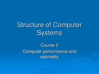
14. Taken 00 01 Not taken 11 10 Branch prediction • Dynamic prediction - take into consideration the history of the branch instructions • Principle: use previous executions of a conditional jump in order to better predict the next executions • Methods: • Next line predictor – stores the pointer to the next instruction (or group of instructions if multiple instructions are fetched in the same time); the method stores the decision as well as the target (pointer) of the branch • Saturating counters – store in 1 or two bits (saturating counters) the decisions made before; in case of 2 bit counter – 4 states: • Strongly not taken (00) – “not taken” is predicted • Weakly not taken (01) – “not taken” is predicted • Weakly taken (10) – “taken” is predicted • Strongly taken (11) - “taken” is predicted • every occurrence of the branch updates the state of the counter

15. Prediction 2 bit counter 0 1 0 0 n bits .... Pattern history table Branch prediction • Dynamic prediction – methods (cont.) • store the decision and the target address for every executed conditional jump in a BHT (Branch History Table) and BTB (Branch Target Buffer); this information will help predict next executions of the same instructions with aprox. 90% probability. • BHT and BTB are indexed with less significant bits of the addresses (of PC); the number of bits used determines the dimension of the tables • Two-level adaptive predictor • necessary for alternating and imbricated conditional jumps • idea: to memorize jump sequence patterns; prediction based on a pattern of taken (1) and not taken (0) branches • a two-level adaptive predictor with an n-bit history can predict any repetitive sequence with any period if all n-bit sub-sequences are different

16. Branch prediction • Dynamic prediction – methods (cont.) • Local branch prediction • a separate history buffer for each conditional jump instruction • it may use a 2 level branch predictor with common or individual pattern history table • Pentium II and III have local branch predictors with a local 4-bit history and a local pattern history table with 16 entries for each conditional jump • Global branch predictor • keeps a shared (global) history of all conditional jumps • any correlation between two branches is used for prediction; • poor results if branches are not correlated; • usually not as good as local predictors • variants: • “gshare" predictor • “gselect” predictor

17. Branch prediction • Dynamic prediction – methods (cont.) • Global branch predictor – possible implementation: two-level adaptive predictor with globally shared history buffer and pattern history table • “gshare" predictor - index in the prediction history table is a XOR between the global history buffer and the jump address • “gselect” predictor – index is obtain by concatenating the history buffer and the jump’s address • Pentium M, Core 2 and AMD processors use global branch prediction • combinations of local and global predictors: • Alloyed branch prediction - concatenates local and global branch history buffer, sometimes also with the address of the jump • Agree predictor – makes a XOR between the local and global predictor (used in Pentium 4) • Hybrid predictor – a combination of predictors; the result is selected through voting or from the predictor with the best hit rates • Loop predictor – detects if a conditional jump is a loop; it is taken N-1 times and not taken 1 time; it may use a counter for the loop; it may be part of a hybrid predictor • Prediction of indirect jumps – when the jump target of a conditional branch has multiple choices – store the previous targets and more bits on the prediction history buffer for such a jump • Prediction of function returns – stores a copy of the stack that contains the return addresses of the executed functions

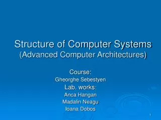
18. Branch address (4 bits) 2-bits per branch local predictors Prediction 2-bit recent global branch history (01 = not taken then taken) Branch prediction • Correlated prediction • example of a combination between local and global prediction • how it works: • every entry in the history table has 4 predictors (e.g. 2 bit counters) • the 2 bit global history buffer select between the 4 predictors • the state of the selected predictor is updated according with the decision made • the global branch history gives the context and the local predictors store behavior of different jump instructions • (2,2) predictor – 2 bit counters and 2 bit history buffer

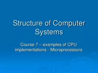
19. 20% 18% 18% 16% 14% 12% 12% 11% 10% Frequency of Mispredictions 8% 6% 6% 6% 6% 5% 5% 4% 4% 2% 1% 1% 0% 0% 0% gcc eqntott 4,096entries: 2-bits per entry Unlimited entries: 2-bits/entry 1,024 entries (2,2) Misprediction statistics for specs tests 1. 4096 Entries 2-bit BHT 2. Unlimited Entries 2-bit BHT 3. 1024 Entries - local and global prediction (2,2) BHT - 1 and 3 require the same amount of memory – 8kbits

20. Branch prediction • Tournament predictor • 2-bit local predictor fail on important branches; by adding global information, performance may improved • Tournament predictors: use two predictors, 1 based on global information and 1 based on local information, and combine with a selector • Hopes to select right predictor for right branch (or right context of branch)

21. 10% 9% 8% Local - 2 bit counters 7% 6% Conditional branch misprediction rate 5% Correlating - (2,2) scheme 4% 3% Tournament 2% 1% 0% 0 8 16 24 32 40 48 56 64 72 80 88 96 104 112 120 128 Total predictor size (Kbits) Misprediction statistics

22. Send PC to memory and branch-target buffer IF Entry found in branch-target buffer? No Yes Send out predicted PC Is instruction a taken branch? No Yes ID Taken Branch? No Yes Normal instruction execution Mispredicted branch, kill fetched instruction; restart fetch at other target; delete entry from target buffer Branch correctly predicted; continue execution with no stalls Enter branch instruction address and next PC into branch-target buffer EX Branch prediction • Branch Target Buffer (BTB): contains target of taken branches • an associative access memory • contains: • jump instr. address • target address • prediction state Jmp addr Target pred PC New address