Download
1 / 45
610 likes | 879 Views
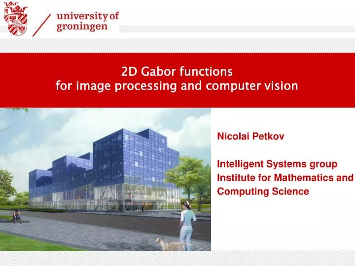
2D Gabor functions f or image processing and computer vision. Nicolai Petkov Intelligent Systems group Institute for Mathematics and Computing Science. Primary v isual cortex ( striate cortex or V1). Brodmann area 17. Wikipedia.org. References to origins - neurophysiology .

E N D
2D Gabor functions for image processing and computer vision Nicolai Petkov Intelligent Systems group Institute for Mathematics and Computing Science
Primary visual cortex (striate cortex or V1) Brodmann area 17 Wikipedia.org
References to origins - neurophysiology Neurophysiology: D.H. Hubel and T.N. Wiesel: Receptive fields, binocular interaction and functional architecture in the cat's visual cortex, Journal of Physiology (London), vol. 160, pp. 106--154, 1962. D.H. Hubel and T.N. Wiesel: Sequence regularity and geometry of orientation columns in the monkey striate cortex, Journal of Computational Neurology, vol. 158, pp. 267--293, 1974. D.H. Hubel: Exploration of the primary visual cortex, 1955-78, Nature, vol. 299, pp. 515--524, 1982.
References to origins - neurophysiology • Hubel and Wiesel named one type of cell "simple" because they shared the following properties: • Their receptive fields have distinct excitatory and inhibitory regions. • These regions follow the summation property. • These regions have mutual antagonism - excitatory and inhibitory regions balance themselves out in diffuse lighting. • It is possible to predict responses to stimuli given the map of excitatory and inhibitory regions.
Receptive field profiles of simple cells Frequency domain Space domain • How are they determined? • recording responses to bars • recording responses to gratings • reverse correlation (spike-triggered average) • Why do simple cells respond to bars and gratings of given orientation?
References to origins – modeling 1D: S. Marcelja: Mathematical description of the responses of simple cortical cells. Journal of the Optical Society of America 70, 1980, pp. 1297-1300. 2D: J.G. Daugman: Uncertainty relations for resolution in space, spatial frequency, and orientation optimized by two-dimensional visual cortical filters, Journal of the Optical Society of America A, 1985, vol. 2, pp. 1160-1169. J.P. Jones and A. Palmer: An evaluation of the two-dimensional Gabor filter model of simple receptive fields in cat striate cortex, Journal of Neurophysiology, vol. 58, no. 6, pp. 1233--1258, 1987
2D Gabor function Frequency domain Space domain
Parametrisation according to: N. Petkov: Biologically motivated computationally intensive approaches to image pattern recognition, Future Generation Computer Systems, 11 (4-5), 1995, 451-465.N. Petkov and P. Kruizinga: Computational models of visual neurons specialised in the detection of periodic and aperiodic oriented visual stimuli: bar and grating cells, Biological Cybernetics, 76 (2), 1997, 83-96.P. Kruizinga and N. Petkov: Non-linear operator for oriented texture, IEEE Trans. on Image Processing, 8 (10), 1999, 1395-1407.S.E. Grigorescu, N. Petkov and P. Kruizinga: Comparison of texture features based on Gabor filters, IEEE Trans. on Image Processing, 11 (10), 2002, 1160-1167.N. Petkov and M. A. Westenberg: Suppression of contour perception by band-limited noise and its relation to non-classical receptive field inhibition, Biological Cybernetics, 88, 2003, 236-246.C. Grigorescu, N. Petkov and M. A. Westenberg: Contour detection based on nonclassical receptive field inhibition, IEEE Trans. on Image Processing, 12 (7), 2003, 729-739.
Preferred spatial frequency and size Space domain Frequency domain Wavelength = 2/512 Frequency = 512/2
Preferred spatial frequency and size Space domain Frequency domain Wavelength = 4/512 Frequency = 512/4
Preferred spatial frequency and size Space domain Frequency domain Wavelength = 8/512 Frequency = 512/8
Preferred spatial frequency and size Space domain Frequency domain Wavelength = 16/512 Frequency = 512/16
Preferred spatial frequency and size Space domain Frequency domain Wavelength = 32/512 Frequency = 512/32
Preferred spatial frequency and size Space domain Frequency domain Wavelength = 64/512 Frequency = 512/64
Orientation Space domain Frequency domain Orientation = 0
Orientation Space domain Frequency domain Orientation = 45
Orientation Space domain Frequency domain Orientation = 90
Symmetry (phase offset) Space domain Space domain Phase offset = 0 (symmetric function) Phase offset = -90 (anti-symmetric function)
Spatial aspect ratio Space domain Frequency domain Aspect ratio = 0.5
Spatial aspect ratio Space domain Frequency domain Aspect ratio = 1
Spatial aspect ratio Space domain Frequency domain Aspect ratio = 2 (does not occur)
Bandwidth Half-response spatial frequency bandwidth b (in octaves)
Preferred spatial frequency and size Space domain Frequency domain Bandwidth = 1 (σ = 0.56 λ) Wavelength = 8/512
Bandwidth Space domain Frequency domain Bandwidth = 0.5 Wavelength = 8/512
Bandwidth Space domain Frequency domain Bandwidth = 2 Wavelength = 8/512
Bandwidth Space domain Frequency domain Bandwidth = 1 (σ = 0.56 λ) Wavelength = 32/512
Bandwidth Space domain Frequency domain Bandwidth = 0.5 Wavelength = 32/512
Bandwidth Space domain Frequency domain Bandwidth = 2 Wavelength = 32/512
Semi-linear Gabor filter What is it useful for? Receptive field G(-x,-y) Output of Convolution followed by half-waverectification Input Ori = 0 Phi = 90 edges Ori = 180 Phi = 90 edges Ori = 0 Phi = 0 lines Ori = 0 Phi = 180 lines bw2 = 2
Bank of semi-linear Gabor filters Which orientations to use Receptive field G(-x,-y) frequency domain Ori = 0 30 60 90 120 150 For filters with s.a.r=0.5 and bw=2, good coverage of angles with 6 orientations
Bank of semi-linear Gabor filters Which orientations to use Input Output Filter in frequency domain Ori = 0 30 60 90 120 150 For filters with sar=0.5 and bw=2, good coverage of angles with 12 orientations
Bank of semi-linear Gabor filters Which orientations to use Result of superposition of the outputs of 12 semi-linear anti-symmetric (phi=90) Gabor filters with wavelength = 4, bandwidth = 2, spatial aspect ratio = 0.5 (after thinning and thresholding lt = 0.1, ht = 0.15).
Bank of semi-linear Gabor filters Which frequencies to use Receptive field G(-x,-y) frequency domain Wavelength = 2 8 32 128 (s.a.r.=0.5) For filters with bw=2, good coverage of frequencies with wavelength quadroppling
Bank of semi-linear Gabor filters Receptive field G(-x,-y) frequency domain Wavelength = 2 4 8 16 32 For filters with bw=1, good coverage of frequencies with wavelength doubling
References to origins - neurophysiology • Complex cells • Their receptive fields do not have distinct excitatory and inhibitory regions. • Response is not modulated by the exact position of the optimal stimulus (bar or grating).
Gabor energy filter Receptive field G(-x,-y) Input Output of Convolution followed by half-waverectification Gabor energy output Ori = 0 Phi = 90 Ori = 180 Phi = 90 Ori = 0 Phi = 0 Ori = 0 Phi = 180
Gabor energy filter Gabor energy output Input Orientation = 0 45 90 135 superposition Result of superposition of the outputs of 4 Gabor energy filters (in [0,180)) with wavelength = 8, bandwidth = 1, spatial aspect ratio = 0.5
Bank of semi-linear Gabor filters How many orientations to use Result of superposition of the outputs of 6 Gabor energy filters (in [0,180)) with wavelength = 4, bandwidth = 2, spatial aspect ratio = 0.5 (after thinning and thresholding lt = 0.1, ht = 0.15).
More efficient detection of intensity changes Space domain Frequency domain dG/dx dG/dy
More efficient detection of intensity changes Gradient magnitude Canny
Contour enhancement by suppression of texture with surround suppression Canny [Petkov and Westenberg, Biol.Cyb. 2003] [Grigorescu et al., IEEE-TIP 2003, IVC 2004]