Download

1 / 46
540 likes | 977 Views
Mass Transfer and Its Applications. Mass transfer – transfer of material from one homogeneous phase to another. Based on differences in vapor pressure, solubility, diffusivity. Driving force for transfer is a concentration difference.

E N D
Mass Transfer and Its Applications • Mass transfer – transfer of material from one homogeneous phase to another. • Based on differences in vapor pressure, solubility, diffusivity. • Driving force for transfer is a concentration difference. • Mass transfer operations – gas absorption, distillation, extraction, leaching, adsorption, crystallization, membrane separations, etc..
Principles of Diffusion • Diffusion – is the movement, under the influence of a physical stimulus, of an individual component through a mixture. • Common cause of diffusion: concentration gradient • Example: Removal of ammonia by gas absorption.
Fick’s Law of Diffusion: • JA = molar flux of comp. A (kg mol/m2.h) • Dv = volumetric diffusivity (m2/h) • cA = concentration (kg mol/m3) • b = distance in direction of diffusion (m)
Mass Transfer Theories • Turbulent flow is desired in most mass-transfer operations: 1. to increase the rate of transfer per unit area 2. to help disperse one fluid in another 3. to create more interfacial area • Mass transfer to a fluid interface is often unsteady-state type.
Mass Transfer Theories Mass transfer coefficient, k • Is defined as rate of mass transfer per unit area per unit conc. difference. • kc is molar flux divided by conc. difference • kc has a unit of velocity in cm/s, m/s • Concentration, c in moles/volume
Mass Transfer Theories Mass transfer coefficient, k • ky in mol/area.time (mol/m2.s) • y or x are mole fractions in the vapor or liquid phase.
MASS TRANSFER THEORIES There are three types of theories in mass transfer coefficients. • Film theories • Penetration theories • Surface –renewal theories
Film Theory • The simplest conceptualization of the gas-liquid transfer process is attributed to Nernst (1904). • Nernst postulated that near the interface there exists a stagnant film . This stagnant film is hypothetical since we really don't know the details of the velocity profile near the interface. • Basic concept – the resistance to diffusion can be considered equivalent to that in stagnant film of a certain thickness • Often used as a basis for complex problems of multicomponent diffusion or diffusion plus chemical reaction.
Mass transfer occurs by molecular diffusion through a fluid layer at phase boundary (solid wall). Beyond this film, concentration is homogeneous and is CAb. • Mass transfer through the film occurs at steady state. • Flux is low and mass transfer occurs at low concentration. Hence,
Integrating Equation (3.55) for the following boundary conditions: CA=CAi when Z=0 CA=CAb when Z=δ We have now:
In this film transport is governed essentially by molecular diffusion. Therefore, Fick's law describes flux through the film.
If the thickness of the stagnant film is given by dn then the gradient can be approximated by: Cb and Ci are concentrations in the bulk and at the interface, respectively.
At steady-state if there are no reactions in the stagnant film there will be no accumulation in the film (Assume that D = constant) -- therefore the gradient must be linear and the approximation is appropriate. And:
Calculation of Ci is done by assuming that equilibrium (Henry's Law) is attained instantly at the interface. (i.e., use Henry's law based on the bulk concentration of the other bulk phase.) Of course this assumes that the other phase doesn't have a "film". This problem will be addressed later. So for the moment: (if the film side is liquid and the opposite side is the gas phase).
A problem with the model is that the effective diffusion coefficient is seldom constant since some turbulence does enter the film area. So the concentration profile in the film looks more like:
Penetration and Surface Renewal Models Most of the industrial processes of mass transfer is unsteady state process. In such cases, the contact time between phases is too short to achieve a stationary state. This non stationary phenomenon is not generally taken into account by the film model. More realistic models of the process have been proposed by Higbie (1935, penetration model) and by Danckwerts ( 1951, surface renewal model). In these models bulk fluid packets (eddies) work their way to the interface from the bulk solution. While at the interface they attempt to equilibrate with the other phase under non-steady state conditions. No film concepts need be invoked. The concentration profile in each eddy ( packet) is determined by the molecular diffusion dominated advective-diffusion equation:
Basic assumptions of the penetration theory are as follows: 1) Unsteady state mass transfer occurs to a liquid element so long it is in contact with the bubbles or other phase 2) Equilibrium exists at gas-liquid interface 3) Each of liquid elements stays in contact with the gas for same period of time Assumption: no advection within the eddy
The solution to this governing equation depends, of course, on boundary conditions. In the Higbie penetration model it is assumed that the eddy does not remain at the surface long enough to affect concentration at the bottom of the eddy ( z = zb). In other words the eddy behaves as a semi-infinite slab. Where C (@ z = zb ) = Cb. Also C (@ z = 0) = Ci .
The boundary conditions are: t = 0, Z > 0 : c = cAb and t > 0, Z = 0 : c = cAi.
Solving the equation with these boundary conditions and then solving for the gradient at z = 0 to get the flux at z = 0 and then finding the average flux over the time the eddy spends on the surface yields the following: q = average time at surface (a constant for a given mixing level). The average mass transfer coefficient during a time interval tcis then obtained by integrating Equation (3.61) as
For the mass transfer in liquid phase, Danckwert (1951) modified the Higbie’s penetration theorywith the surface renewal model. He stated that a portion of the mass transfer surface is replaced with a new surface by the motion of eddies near the surface and proposed the following assumptions: 1) The liquid elements at the interface are being randomly swapped by fresh elements from bulk 2) At any moment, each of the liquid elements at the surface has the same probability of being substituted by fresh element 3) Unsteady state mass transfer takes place to an element during its stay at the interface. s = surface renewal rate (again, a function of mixing level in bulk phase).
Comparison of the models: Higbie and Danckwert's models both predict that J is proportional to D0.5 where the Nernst film model predicts that J is proportional to D. Actual observations show that J is proportional to something in between, D0.5 -1 . There are more complicated models which may fit the experimental data better, but we don't need to invoke them at this time.
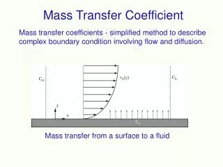
Mass transfer coefficients To simplify calculations we usually define a mass transfer coefficient for either the liquid or gas phase as klor kg(dimensions = L/t).
Boundary Layer Theory • Mass transfer often take place in a thin boundary layer near a surface where the fluid is in laminar flow. • The coefficient, kc depends on 2/3 power of diffusivity and decreases with increasing distance along the surface in the direction of flow • Boundary layer theory can be used to estimate kc for some situations, • but exact prediction of kc cannot be made when the boundary layer become turbulent.
When δ=δ(x)u=Uαand when δ=δm(x)-> u=0.99Uα distance over which solute concentration drops by 99% of (CAi-CAb). where, x is the distance of a point from the leading edge of the plate; kL,xis the local mass transfer coefficient. where, l is the length of the plate.
Two film model In many cases with gas-liquid transfer we have transfer considerations from both sides of the interface. For example, if we invoke the Nernst film model we get the Lewis-Whitman (1923) two-film model as described below.
The same assumptions apply to the two films as apply in the single Nernst film model. The problem, of course, is that we will now have difficulty in finding interface concentrations, Cgi or Cli. We can assume that equilibrium will be attained at the interface (gas solubilization reactions occur rather fast), however, so that:
A steady-state flux balance (okay for thin films) through each film can now be performed. The fluxes are given by: J = kl(Cl -Cli) and J = kg(Cgi-Cg)
If the Whitman film model is used: (Note the Higbie or Danckwerts models can be used without upsetting the conceptualization)
Unfortunately, concentrations at the interface cannot be measured so overallmass transfer coefficients are defined. These coefficients are based on the difference between the bulk concentration in one phase and the concentration that would be in equilibrium with the bulk concentration in the other phase.
Define: Kl = overall mass transfer coefficient based on liquid-phase concentration. Kg = overall mass transfer coefficient based on gas-phase concentration.
Kg,l have dimensions of L/t. Cl* = liquid phase concentration that would be in equilibrium with the bulk gas concentration. = Cg/Hc (typical dimensions are moles/m3). Cg* = gas phase concentration that would be in equilibrium with the bulk liquid concentration. = HcCl (typical dimensions are moles/m3).
Expand the liquid-phase overall flux equation to include the interface liquid concentration.
Then substitute and to get:
In the steady-state, fluxes through all films must be equal. Let all these fluxes be equal to J. On an individual film basis: and
This can be arranged to give: A similar manipulation starting with the overall flux equation based on gas phase concentration will give:
These last two equations can be viewed as "resistance" expressions where 1/Kg or 1/Kl represent total resistance to mass transfer based on gas or liquid phase concentration, respectively.
In fact, the total resistance to transfer is made up of three series resistances: liquid film, interface and gas film. But we assume instant equilibrium at the interface so there is no transfer limitation here. It should be noted that model selection (penetration, surface renewal or film) does not influence the outcome of this analysis.
Single film control It is possible that one of the films exhibits relatively high resistance and therefore dominates the overall resistance to transfer. This, of course, depends on the relative magnitudes of kl, kg and Hc. So the solubility of the gas and the hydrodynamic conditions which establish the film thickness or renewal rate (in either phase) determine if a film controls.
In general, highly soluble gases (low Hc) have transfer rates controlled by gas film (or renewal rate) and vice versa. For example, oxygen (slightly soluble) transfer is usually controlled by liquid film. Ammonia (highly soluble) transfer is usually controlled by gas phase film.
APPLICATIONS Transfer of gas across a gas-liquid interface can be accomplished by bubbles or by creating large surfaces (interfaces). The following are some common applications of gas transfer in treatment process.