Download
1 / 44
440 likes | 441 Views
Learn about the detection of gravitational waves using interferometers such as TAMA, LIGO, LISA, and VIRGO. Explore the science goals, astrophysical sources, and the properties of gravitational waves. Discover how interferometers work and the challenges faced in their detection.

E N D
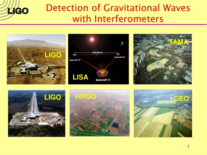
Detection of Gravitational Waves with Interferometers TAMA LIGO LISA VIRGO LIGO GEO
Global network of detectors GEO VIRGO LIGO TAMA AIGO LIGO • Detection confidence • Source polarization • Sky location LISA
Science goals: Detection of gravitational waves • Tests of general relativity • Waves direct evidence for time-dependent metric • Black hole signatures test of strong field gravity • Polarization of the waves spin of graviton • Propagation velocity mass of graviton • Astrophysical processes • Inner dynamics of processes hidden from EM astronomy • Cores of supernovae • Dynamics of neutron stars large scale nuclear matter • The earliest moments of the Big Bang Planck epoch • Astrophysics…
A little bit of GR • From special relativity, “flat” space-time interval is • From general relativity, curved space-time can be treated as perturbation of flat space-timewhere , space-timecurvature flatspace-time metricperturbation
A little bit more GR • Space-time interval becomes • When the gravitational field is weak and in the transverse traceless gauge Einstein’s equations give a wave equation • Space-time tell matter how to moveMatter tells space-time how to curve TT gauge coordinates are marked by world lines of freely falling masses
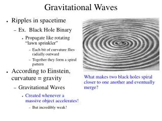
Gravitational waves • Time-dependent solution • h is wave-like motion of the space-time itself ripples of space-time curvature • H is dimensionless • Waves travel at the speed of light • Waves push freely floating objects together and apart stretching and squeezing of space transverse to direction of propagation • Frequency of oscillation is wg
Gravitational waves and GR • Two polarizations • Interaction with matter
DL = h L GWs meet Interferometers • Laser interferometer • Suspend mirrors on pendulums “free” mass
Some properties of gravitational waves • General relativity predicts transverse space-time distortions propagating at the speed of light • In TT gauge and weak field approximation, Einstein field equations wave equation • Conservation laws • Conservation of energy no monopole radiation • Conservation of momentum no dipole radiation • Lowest moment of field quadrupole (spin 2) • Radiated by aspherical astrophysical objects • Radiated by “dark” mass distributions black holes, dark matter
Astrophysics with GWs vs. E&M • Very different information, mostly mutually exclusive • Difficult to predict GW sources based on E&M observations
GWs neutrinos photons now Astrophysical sources of GWs • Coalescing compact binaries • Classes of objects: NS-NS, NS-BH, BH-BH • Physics regimes: Inspiral, merger, ringdown • Periodic sources • Spinning neutron stars ellipticity, precession, r-modes • Burst events • Supernovae asymmetric collapse • Stochastic background • Primordial Big Bang (t = 10-43 sec) • Continuum of sources • The Unexpected
M M h ~10-21 Strength of GWs:e.g. Neutron Star Binary • Gravitational wave amplitude (strain) • For a binary neutron star pair R r
Practical Interferometer • For more practical lengths (L ~ 1 km) a “fold” interferometer to increase phase sensitivity • Df = 2 k DL N (2 k DL); N ~ 100 • Na number of times the photons hit the mirror • Light storage devices a optical cavities • Dark fringe operation a lower shot noise • GW sensitivity P a increase power on beamsplitter • Power recycling • Most of the light is reflected back toward the laser “recycle” light back into interferometer • Price to pay: multiple resonant cavities whose lengths must be controlled to ~ 10-8l
Power-recycled Interferometer Optical resonance: requires test masses to be held in position to 10-10-10-13meter“Locking the interferometer” end test mass Light bounces back and forth along arms ~100 times 30 kW Light is “recycled” ~50 times 300 W input test mass Laser + optical field conditioning signal 6Wsingle mode
3 0 3 ( ± 0 1 k 0 m m s ) LIGO WA 4 km (H1) 2 km (H2) LA 4 km(L1)
Initial LIGO Sensitivity Goal • Strain sensitivity < 3x10-23 1/Hz1/2at 200 Hz • Displacement Noise • Seismic motion • Thermal Noise • Radiation Pressure • Sensing Noise • Photon Shot Noise • Residual Gas • Facilities limits much lower
Limiting Noise Sources:Seismic Noise • Motion of the earth few mm rms at low frequencies • Passive seismic isolation ‘stacks’ • amplify at mechanical resonances • but get f-2 isolation per stage above 10 Hz
FRICTION Limiting Noise Sources:Thermal Noise • Suspended mirror in equilibrium with 293 K heat bath akBT of energy per mode • Fluctuation-dissipation theorem: • Dissipative system will experience thermally driven fluctuations of its mechanical modes: Z(f) is impedance (loss) • Low mechanical loss (high Quality factor) • Suspension no bends or ‘kinks’ in pendulum wire • Test mass no material defects in fused silica
Limiting Noise Sources:Quantum Noise • Shot Noise • Uncertainty in number of photons detected a • Higher input power Pbsa need low optical losses • (Tunable) interferometer response Tifo depends on light storage time of GW signal in the interferometer • Radiation Pressure Noise • Photons impart momentum to cavity mirrorsFluctuations in the number of photons a • Lower input power, Pbs Optimal input power for a chosen (fixed) Tifo
Operations Strategy • Interferometer performance • Intersperse commissioning and data taking consistent with obtaining one year of integrated data at h = 10-21 by end of 2006 • Astrophysical searches • Two “upper limit” runs S1 and S2 (at unprecedented early sensitivity) are interleaved with commissioning • S1 Aug-Sep 2002 duration: 2 weeks • S2 Feb-Apr 2003 duration: 8 weeks • First search run (S3) planned for late 2003 (duration: 6 months) • Finish detector integration & design updates... • Engineering "shakedown" runs interspersed as needed • Advanced LIGO
H1: 235 hrs H2: 298 hrs L1: 170 hrs 3X: 95.7 hrs Red lines: integrated up timeGreen bands (w/ black borders): epochs of lock S1 Run Summary • August 23 – September 9, 2002: 408 hrs (17 days). • H1 (4km): duty cycle 57.6% ; Total Locked time: 235 hrs • H2 (2km): duty cycle 73.1% ; Total Locked time: 298 hrs • L1 (4km): duty cycle 41.7% ; Total Locked time: 170 hrs • Double coincidences: • L1 && H1 : duty cycle 28.4%; Total coincident time: 116 hrs • L1 && H2 : duty cycle 32.1%; Total coincident time: 131 hrs • H1 && H2 : duty cycle 46.1%; Total coincident time: 188 hrs Triple Coincidence: L1, H1, and H2 : duty cycle 23.4% ; total 95.7 hours
Strain Sensitivities During S1 H2 &H1 L1 3*10-21 Hz -1/2@ f ~300 Hz
Summary of upper limits for S1 • Upper limits as presented at AAAS meeting Feb 2003 • Stochastic backgrounds • Upper limit 0 < 72.4(H1- H2 pair) • Neutron star binary inspiral • Range of detectability < 200 kpc(1.4 – 1.4 MSUN NS binary with SNR = 8) • Coalescence Rate for Milky Way equivalent galaxy < 164 /yr 90% CL • Periodic sources PSR J1939+2134 at 1283 Hz • GW radiation h < 2 10-22 90% CL (expect h ~ 10-27 if pulsar spindown entirely due GW emission) • Burst sources • Upper limit h < 5 10-17 90% CL • S2 is ~10x more sensitive and ~4x longer Standard Inflation Prediction < 10-15 Limit from Big Bang Nucleosynthesis < 10-4
Strain Sensitivity coming into S2 L1 S1 6 Jan
LIGO Science Has Started • LIGO has started taking data • First science run (S1) last summer • Collaboration has carried out first analysislooking for • Bursts • Compact binary coalescences • Stochastic background • Periodic sources • Second science run (S2) ended last week • Sensitivity is ~10x better than S1 • Duration is ~ 4x longer • Bursts4x lower rate limit & 10x lower strain limit • Inspirals reach > 1 Mpc -- includes M31 (Andromeda) • Stochastic background limits on WGW < 10-2 • Periodic sources limits on hmax ~ few x 10-23 (e ~ few x 10-6 @ 3.6 kpc)
The next-generation detectorAdvanced LIGO (aka LIGO II) • Now being designed by the LIGO Scientific Collaboration • Goal: • Quantum-noise-limited interferometer • Factor of ten increase in sensitivity • Factor of 1000 in event rate. One day > entire2-year initial data run • Schedule: • Begin installation: 2006 • Begin data run: 2008
Quantum LIGO I LIGO II Test mass thermal Suspension thermal Seismic A Quantum Limited Interferometer • Facility limits • Gravity gradients • Residual gas • (scattered light) • Advanced LIGO • Seismic noise 4010 Hz • Thermal noise 1/15 • Optical noise 1/10 • Beyond Adv LIGO • Thermal noise: cooling of test masses • Quantum noise: QND
f i (l) r(l).e Power Recycling l Signal Recycling Optimizing the optical response: Signal Tuning Cavity forms compound output coupler with complex reflectivity. Peak response tuned by changing position of SRM Reflects GW photons back into interferometer to accrue more phase
Thorne… Advance LIGO Sensitivity:Improved and Tunable
Thorne Detection of candidate sources
~10 min 20 Mpc ~3 sec 300 Mpc Implications for source detection • NS-NS Inpiral • Optimized detector response • NS-BH Merger • NS can be tidally disrupted by BH • Frequency of onset of tidal disruption depends on its radius and equation of state a broadband detector • BH-BH binaries • Merger phase non-linear dynamics of highly curved space time a broadband detector • Supernovae • Stellar core collapse neutron star birth • If NS born with slow spin period (< 10 msec) hydrodynamic instabilities a GWs
Sco X-1 Signal strengths for 20 days of integration Source detection • Spinning neutron stars • Galactic pulsars: non-axisymmetry uncertain • Low mass X-ray binaries:If accretion spin-up balanced by GW spin-down, then X-ray luminosity GW strengthDoes accretion induce non-axisymmetry? • Stochastic background • Can cross-correlate detectors (but antenna separation between WA, LA, Europe a dead band) • WGW(f ~ 100 Hz) = 3 x 10⁻⁹ (standard inflation 10-15) (primordial nucleosynthesis d 10-5) (exotic string theories 10-5) Thorne GW energy / closure energy
LISA - The Overview • Concept • 3 spacecraft constellation separated by 5 x10⁶ km. • Earth-trailing solar orbit • Drag-free proof masses • Interferometry to measure changes in distance between masses caused by gravitational waves • Partnership between ESA, JPL and GSFC • Science Goals • Observe and measure the rate of massive and super-massive black hole mergers to high red shift • Observe the inspiral and merger of compact stellar objects into massive black holes • Detect gravitational radiation from compact binary star systems in our galaxy • Observe gravitational radiation from the early universe
Astrophysical Sources • Mapping the gravitational wave sky between 0.1 mHz and 1 Hz will be an exploration of astrophysical systems involving compact objects such as • Supermassive black holes (105-107 M) • Intermediate mass black holes (102-105 M) • Stellar mass black holes (1-102 M) • Neutron stars (~1.4 M) • White dwarfs ( 1 M) . . . which are rapidly accelerated in non-spherical mass distributions, typically close binary systems • Some of these objects may not radiate Other unexpected objects may exist
Binary Inspiral Sensitivity • Waveforms from slow motion (pN) approx. • Measure: • Inspiral rate “chirp mass” • Relativistic effects component masses • Amplitude luminosity distance • Polarization (network) inclination • Timing (network) sky position • Rates estimated from • Empirical estimates based on observed binaries • Sensitive to faint pulsar population • Stellar evolution/dynamics models • Sensitive to formation channels, stellar winds, supernova kick velocities, etc. NS/NS @ 10Mpc BBH (40M)500 Mpc binary neutron stars binary black holes V Kalogera et al, Astrophys J 556 340 (2000) S Portegies Zwart, S McMillan, Astrophys J 528 L17 (2000)
Unmodeled Burst SourcesSupernovae and Core Collapse Hang-up at 100km, D=10kpc SN1987A Hang-up at 20km, D=10kpc Proto neutron star boiling
Crab pulsar limit (4 month observation) Hypothetical population of young, fast pulsars (4 months @ 10 kpc) Crustal strain limit (4 months @ 10 kpc) Sco X-1 to X-ray flux (1 day) PSR J1939+2132 (4 month observation) Sensitivity to Pulsars
Cosmic Microwave Background Primordial Gravitational-Wave Background Stochastic Background Background ?
Ω = 10-5 (4 month observation) Overlap Reduction LHO-LLO Stochastic Background Sensitivity • Fraction of energy density in Universe in gravitational waves: • Constraint from nucleosynthesis: • More recent processes may also produce stochastic backgrounds