Download
1 / 49
490 likes | 492 Views
Learn about the definitions and properties of graphs, including adjacency, paths, cycles, connectedness, and weighted graphs. Explore examples and implementations using adjacency matrices and lists.

E N D
GRAPH – Definitions • A graph G = (V, E) consists of • a set of vertices, V, and • a set of edges, E, where each edge is a pair (v,w) s.t. v,w V • Vertices are sometimes called nodes, edges are sometimes called arcs. • If the edge pair is ordered then the graph is called a directed graph (also calleddigraphs). • We also call a normal graph (which is not a directed graph) an undirected graph. • When we say graph we mean that it is an undirected graph.
Graph – Definitions • Two vertices of a graph are adjacent if they are joined by an edge. • Vertex w is adjacent to v iff (v,w) E. • In an undirected graph with edge (v, w) and hence (w,v) w is adjacent to v and v is adjacent to w. • A path between two vertices is a sequence of edges that begins at one vertex and ends at another vertex. • i.e. w1, w2, …, wN is a path if (wi, wi+1) E for 1 i . N-1 • A simple path passes through a vertex only once. • A cycle is a path that begins and ends at the same vertex. • A simple cycle is a cycle that does not pass through other vertices more than once.
1 2 4 5 3 Graph – An Example A graph G (undirected) The graph G= (V,E) has 5 vertices and 6 edges: V = {1,2,3,4,5} E = { (1,2),(1,3),(1,4),(2,5),(3,4),(4,5), (2,1),(3,1),(4,1),(5,2),(4,3),(5,4) } • Adjacent: 1 and 2 are adjacent -- 1 is adjacent to 2 and 2 is adjacent to 1 • Path: 1,2,5 ( a simple path), 1,3,4,1,2,5 (a path but not a simple path) • Cycle: 1,3,4,1 (a simple cycle), 1,3,4,1,4,1 (cycle, but not simple cycle)
connected disconnected complete Graph -- Definitions • A connected graph has a path between each pair of distinct vertices. • A complete graph has an edge between each pair of distinct vertices. • A complete graph is also a connected graph. But a connected graph may not be a complete graph.
Directed Graphs • If the edge pair is ordered then the graph is called a directed graph (also calleddigraphs). • Each edge in a directed graph has a direction, and each edge is called a directed edge. • Definitions given for undirected graphs apply also to directed graphs, with changes that account for direction. • Vertex w is adjacent to v iff (v,w) E. • i.e. There is a direct edge from v to w • w is successor of v • v is predecessor of w • A directed path between two vertices is a sequence of directed edges that begins at one vertex and ends at another vertex. • i.e. w1, w2, …, wN is a path if (wi, wi+1) E for 1 i . N-1
Directed Graphs • A cycle in a directed graph is a path of length at least 1 such that w1 = wN. • This cycle is simple if the path is simple. • For undirected graphs, the edges must be distinct • A directed acyclic graph (DAG) is a type of directed graph having no cycles. • An undirected graph is connected if there is a path from every vertex to every other vertex. • A directed graph with this property is called strongly connected. • If a directed graph is not strongly connected, but the underlying graph (without direction to arcs) is connected then the graph is weakly connected.
1 2 4 5 3 Directed Graph – An Example The graph G= (V,E) has 5 vertices and 6 edges: V = {1,2,3,4,5} E = { (1,2),(1,4),(2,5),(4,5),(3,1),(4,3) } • Adjacent: 2 is adjacent to 1, but 1 is NOT adjacent to 2 • Path: 1,2,5 ( a directed path), • Cycle: 1,4,3,1 (a directed cycle),
1 2 1 2 4 5 3 4 5 3 Weighted Graph • We can label the edges of a graph with numeric values, the graph is called a weighted graph. 8 Weighted (Undirected) Graph 6 10 3 5 7 8 Weighted Directed Graph 6 10 3 5 7
Graph Implementations • The two most common implementations of a graph are: • Adjacency Matrix • A two dimensional array • Adjacency List • For each vertex we keep a list of adjacent vertices
Adjacency Matrix • An adjacency matrix for a graph with n vertices numbered 0,1,...,n-1 is an n by n array matrix such that matrix[i][j] is 1 (true) if there is an edge from vertex i to vertex j, and 0 (false) otherwise. • When the graph is weighted, we can let matrix[i][j] be the weight that labels the edge from vertex i to vertex j, instead of simply 1, and let matrix[i][j] equal to instead of 0 when there is no edge from vertex i to vertex j. • Adjacency matrix for an undirected graph is symmetrical. • i.e. matrix[i][j] is equal to matrix[j][i] • Space requirement O(|V|2) • Acceptable if the graph is dense.
A directed graph Its adjacency matrix Adjacency Matrix – Example1
Adjacency Matrix – Example2 Its Adjacency Matrix An Undirected Weighted Graph
Adjacency List • An adjacency list for a graph with n vertices numbered 0,1,...,n-1 consists of n linked lists. The ith linked list has a node for vertex j if and only if the graph contains an edge from vertex i to vertex j. • Adjacency list is a better solution if the graph is sparse. • Space requirement is O(|E| + |V|), which is linear in the size of the graph. • In an undirected graph each edge (v,w) appears in two lists. • Space requirement is doubled.
A directed graph Its Adjacency List Adjacency List – Example1
An Undirected Weighted Graph Its Adjacency List Adjacency List – Example2
Adjacency Matrix vs Adjacency List • Two common graph operations: • Determine whether there is an edge from vertex i to vertex j. • Find all vertices adjacent to a given vertex i. • An adjacency matrix supports operation 1 more efficiently. • An adjacency list supports operation 2 more efficiently. • An adjacency list often requires less space than an adjacency matrix. • Adjacency Matrix: Space requirement is O(|V|2) • Adjacency List : Space requirement is O(|E| + |V|), which is linear in the size of the graph. • Adjacency matrix is better if the graph is dense (too many edges) • Adjacency list is better if the graph is sparse (few edges)
Graph Traversals • A graph-traversal algorithm starts from a vertex v, visits all of the vertices that can be reachable from the vertex v. • A graph-traversal algorithm visits all vertices if and only if the graph is connected. • A connected component is the subset of vertices visited during a traversal algorithm that begins at a given vertex. • A graph-traversal algorithm must mark each vertex during a visit and must never visit a vertex more than once. • Thus, if a graph contains a cycle, the graph-traversal algorithm can avoid infinite loop. • We look at two graph-traversal algorithms: • Depth-First Search (aka Depth-First Traversal) • Breadth-First Search (aka Breadth-First Traversal)
Depth-First Search • For a given vertex v, the depth-first search algorithm proceeds along a path from v as deeply into the graph as possible before backing up. • That is, after visiting a vertex v, the depth-first search algorithm visits (if possible) an unvisited adjacent vertex to vertex v. • The depth-first traversal algorithm does not completely specify the order in which it should visit the vertices adjacent to v. • We may visit the vertices adjacent to v in sorted order.
Depth-First Search – Example • A depth-first search of the graph starting from vertex v. • Visit a vertex, then visit a vertex adjacent to that vertex. • If there is no unvisited vertex adjacent to visited vertex, back up to the previous step.
Recursive Depth-First Search Algorithm dfs(in v:Vertex) { // Traverses a graph beginning at vertex v // by using depth-first strategy // Recursive Version Mark v as visited; for (each unvisited vertex u adjacent to v) dfs(u) }
Iterative Depth-First Search Algorithm dfs(in v:Vertex) { // Traverses a graph beginning at vertex v // by using depth-first strategy: Iterative Version s.createStack(); // push v into the stack and mark it s.push(v); Mark v as visited; while (!s.isEmpty()) { if (no unvisited vertices are adjacent to the vertex on the top of stack) s.pop(); // backtrack else { Select an unvisited vertex u adjacent to the vertex on the top of the stack; s.push(u); Mark u as visited; } } }
2 1 3 8 9 6 4 5 7 Trace of Iterative DFS – starting from vertex a
Breadth-First Search • After visiting a given vertex v, the breadth-first search algorithm visits every vertex adjacent to v that it can before visiting any other vertex. • The breadth-first traversal algorithm does not completely specify the order in which it should visit the vertices adjacent to v. • We may visit the vertices adjacent to v in sorted order.
Breadth-First Search– Example • A breadth-first search of the graph starting from vertex v. • Visit a vertex, then visit all vertices adjacent to that vertex.
Iterative Breadth-First Search Algorithm bfs(in v:Vertex) { // Traverses a graph beginning at vertex v // by using breath-first strategy: Iterative Version q.createQueue(); // add v to the queue and mark it q.enqueue(v); Mark v as visited; while (!q.isEmpty()) { q.dequeue(w); for (each unvisited vertex u adjacent to w) { Mark u as visited; q.enqueue(u); } } }
2 1 5 9 4 6 8 7 3 Trace of Iterative BFT – starting from vertex a
d b e a h c f g Exercise a) Give the sequence of vertices when they are traversed starting from the vertex a using the depth-first search algorithm. b) Give the sequence of vertices when they are traversed starting from the vertex a using the breadth-first search algorithm.
Some Graph Algorithms • Shortest Path Algorithms • Unweighted shortest paths • Weighted shortest paths (Dijkstra’s Algorithm) • Topological sorting • Network Flow Problems • Minimum Spanning Tree • Depth-first search Applications
Unweighted Shortest-Path problem • Find the shortest path (measured by number of edges) from a designated vertex S to every vertex. 1 2 4 5 3 6 7
Algorithm • Start with an initial node s. • Mark the distance of s to s, Ds as 0. • Initially Di = for all i s. • Traverse all nodes starting from s as follows: • If the node we are currently visiting is v, for all w that are adjacent to v: • Set Dw = Dv + 1 if Dw = . • Repeat step 2.1 with another vertex u that has not been visited yet, such that Du = Dv (if any). • Repeat step 2.1 with another unvisited vertex u that satisfies Du = Dv +1.(if any)
Figure 14.21A Searching the graph in the unweighted shortest-path computation. The darkest-shaded vertices have already been completely processed, the lightest-shaded vertices have not yet been used as v, and the medium-shaded vertex is the current vertex, v. The stages proceed left to right, top to bottom, as numbered (continued).
Figure 14.21B Searching the graph in the unweighted shortest-path computation. The darkest-shaded vertices have already been completely processed, the lightest-shaded vertices have not yet been used as v, and the medium-shaded vertex is the current vertex, v. The stages proceed left to right, top to bottom, as numbered.
Unweighted shortest path algorithm void Graph::unweighted_shortest_paths(vertex s) { //An application of BFS: Finding the shortest path between //two nodes u and v, with path length measured by # of edges Queue<Vertex> q; Vertex v,w; for each Vertex v v.dist = INFINITY; s.dist = 0; q.enqueue(s); while (!q.isEmpty()) { v= q.dequeue(); v.known = true; // not needed anymore for each w adjacent to v if (w.dist == INFINITY) { w.dist = v.dist + 1; w.path = v; q.enqueue(w); } } }
Weighted Shortest-path Problem • Find the shortest path (measured by total cost) from a designated vertex S to every vertex. All edge costs are nonnegative. 2 1 2 4 10 3 1 2 4 5 3 2 8 4 5 2 1 6 7
Weighted Shortest-path Problem • The method used to solve this problem is known as Dijkstra’s algorithm. • An example of a greedy algorithm • Use the local optimum at each step • Solution is similar to the solution of unweighted shortest path problem. • The following issues must be examined: • How do we adjust Dw? • How do we find the vertex v to visit next?
Figure 14.23 The eyeball is at v and w is adjacent, so Dw should be lowered to 6.
Dijkstra’s algorithm • The algorithm proceeds in stages. • At each stage, the algorithm • selects a vertex v, which has the smallest distance Dv among all the unknown vertices, and • declares that the shortest path from s to v is known. • then for the adjacent nodes of v (which are denoted as w) Dw is updated with new distance information • How do we change Dw? • If its current value is larger than Dv + c v,w we change it.
Figure 14.25A Stages of Dijkstra’s algorithm. The conventions are the same as those in Figure 14.21 (continued).
Figure 14.25B Stages of Dijkstra’s algorithm. The conventions are the same as those in Figure 14.21.
Implementation • A queue is no longer appropriate for storing vertices to be visited. • The priority queue is an appropriate data structure. • Add a new entry consisting of a vertex and a distance, to the priority queue every time a vertex has its distance lowered.
Shortest Paths: Dijkstra’s Algorithm PriorityQueue<Vertex> pq; For each node v { v.dist = ∞; v.path = null; } s.dist = 0; add all vertices to pq; while(!pq.isEmpty()) {O(V) Vertex v = pq.deleteMin();//O(logV), O(V) if arrayused for each edge(v,w) //O(E) alt = v.dist + weight(v,w); if (alt < w.dist) { update w.dist = v.dist + weight(v,w); w.path = v; pq.decrease_priority(w,alt);//O(logV) //Amortized O(1) if Fibonacci heap used //O(1) if array used }}}
Shortest Paths: Dijkstra’s Algorithm Analysis: • With priority queue: O(|V|log|V|+|E|log|V|) O(|E|log|V|) O(|V|log|V|+|E|) //with Fibonacci heap • Without priority queue (e.g., array): O(|V|2 + |E|) O(|V|2)
Topological Sorting • A topological sortof a dag G = (V, E) is a linear ordering of all its vertices such that if G contains an edge (u, v), then u appears before v in the ordering. (If the graph is not acyclic, then no linear ordering is possible.) • A topological sort of a graph can be viewed as an ordering of its vertices along a horizontal line so that all directed edges go from left to right. • Different from the usual kind of Sorting we studied before
Topological Sorting • Prof. Yusuf topologically sorts his clothing when getting dressed
Topological Sorting • TOPOLOGICAL-SORT(G) Call DFS(G) to compute finishing times f [v] for each vertex v As each vertex is finished, insert it onto the front of a linked list return the linked list of vertices
Topological Sorting Analysis: TOPOLOGICAL-SORT(G)takes O(|V| + |E|) time as DFS takes O(|V| + |E|) and insertion to list takes O(1) for each |V| vertices
Topological Sorting Applications (other than dressing you up) • Resolving dependencies • To build dll A, you must have built DLLs B, C an D (Maybe you have a reference of B,C and D in the project that builds A). You mark a dependency edge from each of B, C and D to A implying that A depends on the other three and can only be built once each of the three are built. After constructing a graph of these dlls and dependency edges, you can conclude that a successful build is possible iff the resulting graph is acyclic. How does the build system decide in which order to build these dlls? It sorts them topologically. Therefore, in an order like X->Z->T->B->D->C->A, it can start building X (which may only depend on external assemblies already built), then follow the topologically sorted list of assemblies. • Many other task scheduling jobs