Download
1 / 15
170 likes | 669 Views
Three Models of Aggregate Supply. The sticky wage, imperfect-information, and sticky price models. Model Background. Most economists analyze short-run fluctuations in aggregate income and the price level using the AD/AS model.

E N D
Three Models of Aggregate Supply The sticky wage, imperfect-information, and sticky price models.
Model Background • Most economists analyze short-run fluctuations in aggregate income and the price level using the AD/AS model. • Earlier we introduced long-run AS as a vertical line which implied perfect flexibility for prices. • Our short-run AS curve was perfectly horizontal which implied perfect rigidity for prices. • Now we will propose theories for a positively sloped AS curve. This implies a tradeoff between between inflation and unemployment. • All three models adhere to the following functional form. where α>0, Y is output, is the natural rate of output, P is the price level, and Pe is the expected price level.
Model Background • This equation states that output deviates from its natural rate when the price level deviates from the expected price level. α indicates how much output responds to unexpected changes in P and 1/α is the slope of the AS curve. • Although each of the three theories adheres to the given functional form, each highlights a different reason why unexpected movements in the price level are associated with fluctuations in aggregate output.
The Sticky Wage Model W/P • Many economists believe that nominal wages are sticky in the short run. When the nominal wage is stuck, a rise in P from P0 to P1 lowers the real wage, making labour cheaper. The lower real wage induces firms to hire more labour. W/P0 W/P1 DL The additional labour hired produces more output. The positive relationship between P and Y means AS slopes upward. L L0 L1 Y P Y1 Y=F(L) P1 Y0 P0 L Y L0 L1 Y0 Y1
The Sticky Wage Model • The downfall of the sticky wage model is that it predicts a countercyclical relationship between the real wage and output. Actual data suggests a procyclical relationship.
The Imperfect-Information Model • Unlike the sticky wage model, this model assumes that wages and prices are free to adjust and that the labour market clears. The imperfect-information model attributes the positively sloped AS curve to temporary misperceptions about prices.
The Imperfect-Information Model • With some simple algebra we can rewrite our supply curve in inverse form getting… Each individual supplier observes their own price closely… …but must guess at the overall price level and form an expectation. P If all prices in the economy (unobserved) increase including the supplier’s own price (observed) and the supplier expected it then P=Pe and output remains unchanged. The perception is that the relative price for the supplier has not changed. P1=P1e P0=P0e Y Y0
The Imperfect-Information Model If all prices in the economy (unobserved) increase including the supplier’s own price (observed) and the supplier did not expect it then the supplier perceives mistakenly that the relative price of their own product has increased (P>Pe). The supplier then produces more output. P P1>P1e P0=P0e Y Y0 Y1 So, when actual prices exceed expected prices, suppliers raise their output. The positive relationship between P and Y means AS slopes upward.
The Sticky Price Model • This model explains an upward sloping AS curve by assuming that some prices are sticky because • firms have long term contracts with customers, • firms hold prices steady in order not to annoy regular customers with frequent price changes, and • for firms who have printed and distributed a catalog or price list it is too costly to alter prices.
The Sticky Price Model • The typical firm’s desired price “p” depends on two macroeconomic variables… The overall price level “P”, where a higher price level implies that the firm’s costs are higher so the firm wants to charge more for its own product. And the level of aggregate income “Y”, where a higher level of income raises the demand for the firm’s product so firms raise prices to cover the higher marginal costs. The parameter “a” measures how much the firm’s desired price responds to the level of aggregate output.
The Sticky Price Model • Now we assume there are two types of firms. Some have flexible prices. They always set their prices according to this equation. Others have sticky prices. They announce their prices in advance based on what they expect economic conditions to be. For simplicity, assume that these firms expect output to be at its natural rate, so that the last term is zero. These firms set their price based on what they expect other firms to charge.
The Sticky Price Model • With the pricing rules of these two groups we can derive the aggregate supply equation. • We want the overall price level in the economy, which is the weighted average of the prices set by the two groups. If “s” is the fraction of firms with sticky prices and “1 – s” the fraction with flexible prices, then the overall price level is… The first term is the price of the sticky-price firms weighted by their fraction in the economy. The second term is the price of the flexible price firms weighted by their fraction. Now subtract (1 – s)P from both sides getting… Dividing both sides by “s” gives us…
The Sticky Price Model • So when firms expect a high price level, they expect high costs. Those firms that fix prices in advance set their prices high. These high prices cause the other firms to set high prices also. Hence, a high expected price level Pe leads to a high actual price level P. • When output is high, the demand for goods is high. Those firms with flexible prices set their prices high, which leads to a high price level. The effect of output on the price level depends on the proportion of firms with flexible prices. • So, the overall price level depends on the expected price level and on the level of output. Algebraic rearrangement of the price formula… Yields the familiar AS function. Where...
The Sticky Price Model W/P • Like the other models the sticky-price model says that the deviation of output from the natural rate is positively associated with the deviation of the price level from the expected price level. • The sticky price model is also consistent with a procyclical real wage. SL W/P DL If a firm’s price is stuck in the short run then a decrease in AD reduces the amount the firm is able to sell. The firm responds by reducing demand for labour. L P L1 L0 So fluctuations in output are associated with a shifting labour demand curve. P1 If a firm’s price is flexible in the short run then a decrease in AD reduces the amount the firm is able to sell. The firm responds by reducing its price. P0 Y Y1 Y0
Conclusion • This section presents three models of AS that why it is upward sloping in the short run. One model assumes nominal wages are sticky; the second assumes information about prices is imperfect; the third assumes prices are sticky. The world may contain all three of these market imperfections, and all may contribute to the behavior of short-run AS. All can be summarized by the equation…