Download
1 / 41
410 likes | 613 Views
Animating Sand as a Fluid. Yongning Zhu Robert Bridson Presented by KKt. Abstract. Physics-based simulation method for animating sand Existing water simulator can be turned into a sand simulator Alternative method for simulating fluids Issue of reconstructing a surface from particle.

E N D
Animating Sand as a Fluid Yongning Zhu Robert Bridson Presented by KKt
Abstract • Physics-based simulation method for animating sand • Existing water simulator can be turned into a sand simulator • Alternative method for simulating fluids • Issue of reconstructing a surface from particle
Introduction • We wanted to animating granular materials • sand, gravel, grains, soil, rubble, flour, sugar • We think sand as a continuous material • How should it respond to force? • The purposes of plausible animation we simplify the exist models • We combine grids and particles • We reconstruct a smooth surface
Related Work • Miller and Pearce[1989] • Simple particle system model • Later Luciani et al.[1995] • Particle system model specifically for granular materials • Li and Moshell[1993] • Dynamic height-field simulation of soil with Mohr-Coulomb constitutive model • Sumner et al.[1998] • Height-field approach with simple displacement and erosion rules • Onoue and Nishita[2003] • multi-valued height-fields
Particles for water simulation • Desbrun and Cani[1996] • Smooth Particle Hydrodynamics • Müller et al.[2003] • SPH further for water simulation • Premoze et al.[2003] • Used variation on SPH with an approximate projection • Takeshita et al.[2003] • For fire
Grids for water simulation • Foster and Metaxas[1996] • Grid-based fully 3D water simulation in graphics • Stam[1999] • Semi-Lagrangian advection method for faster simulation • Foster and Fedkiw[2001] • Level set and marker particles • Losasso et al.[2004] • Adapted octree grids • Hong and Kim[2003] • Volume-of-fluid algorithms
Plastic flow • Terzopoulos and Fleischer[1988] • First introduced plasticity to physics-based animation • O’Brien et al.[2002] • Fracture-capable tetrahedral-mesh finite element simulation • Müller and Gross [2004] • Real-time elastic simulation • Jaeger et al.[1996] • Scientific description of the physics of granular materials • Elasto-plastic finite element formulation with Mohr-Coulomb or Drucker-Prager yield conditions
PIC and FLIP • Harlow[1963] • Particle-in-cell(PIC) for compressible flow • Harlow and Welch[1965] • Marker-and-cell for incompressible flow • Brackbill and Ruppel[1986] • Fluid-Implicit-Particle (FLIP)
Sand Modeling • Frictional Plasticity • Mohr-Coulomb law • Material will not yield • |..|F is Frobenius norm • φ is friction angle • If is big enough, do not shear • cf.
Basic mathematics • Trace • Frobenius norm σ is the singular values of A
Stress • A measure of the average amount of force exerted per unit area • σ is the average stress P is the force, A is area • Stress is consisted of • Normal stress σ • Shearing stress τ
Terminologies <Stress energy tensor> <Von Mises stress in 2D> <Von Mises and Tresca Yield surfaces in principle stress coordinates>
Yielding sand flow • direction • That the shearing force is pushing • Nonassociated to gradient of yielding • Normal ways are not proper here • Because of lack of dilation • A little when it begins to flow • Stops as soon as the sand is freely flowing
A Simplified Model • Ignore the nearly imperceptible elastic deformation • Tiny volume changes • Decompose regions two • Rigid moving • incompressible shearing flow • Pressure required to make entire velocity field incompressible • Certainly false but for plausible results
Frictional stress • Neglecting elastic effects • At sand is flowing area • Strain rate : • At the yield surface • that most directly resists the sliding
Strain • ε은 측정방향으로의 strain • lo은 물질의 기본 길이, l은 현재 길이 • Shear strain • Strain tensor
Yield condition • Without elastic stress and strain • Stop all sliding motion in a time step • : Newton’s law • Divide with area
Simulation algorithm • Advection • Usual water solver • Gravity, boundary condition, pressure • Subtract for incompressible • Evaluate the strain rate tensor D, according to yield condition • If < rigid store • Else solid store • According to regions • Project connected rigid groups • Others velocity
n u·n u uT Boundary Frictional Boundary Conditions • Important behavior • Don’t sliding at vertical surfaces • Always allow sliding never be stable
Cohesion • c > 0 is the cohesion coefficient • Appropriate for soil or sticky materials • Improving results • With very small amount of cohesion
Fluid Simulation Revisited • Grids and Particles • Grid-based methods (Eulerian grids) • Store on a fixed grid • velocity, pressure, some sort of indicator • Where the fluid is or isn’t • Staggered “MAC” grid is used • Particle-based methods • SPH(Smoothed Particle Hydrodynamics) • Actual chunks and motion of fluid are achieved by moving the particles themselves • Navier-Stokes equations • Governing equation
Grid-based methods • Primary strength • Simplicity of the discretization • Incompressibility condition • Weakness • Difficult to advection • Semi-Lagrangian • Excessive numerical dissipation • Interpolation error • Levelset and VOF(volume-of-fluid) • Advection and time consuming
Particle-based methods • Strong point • Advection with excellent accuracy • With Ordinary Differential Equation (ODE) • Weak point • Pressure and incompressibility condition • Time step • Particle-level set method • Highest fidelity water animations • Particles can be exploited even further • Simplifying and accelerating, affording new benefits
Particle-in-Cell Methods • PIC • Simulating compressible flow • Handled advection with particles • But everything else on a grid • FLIP (Fluid Implicit Particle) • Correct numerical dissipation
Save difference & Correct ERROR! PIC vs FLIP
PIC steps • Initialize particle positions & velocities • For each time step: • Interpolate particle velocity to grid • Do all non-advection steps of water simulation • Interpolate the new grid velocity to the particles • Move particles with ODE, and satisfy boundary • Output the particle position • There is no grid-based advection, or vorticity confinement and particle-level
FLIP steps • Initialize particle positions & velocities • For each time step: • Interpolate particle velocity to grid • Save the grid velocities • Do all non-advection steps of water simulation • Subtract new grid vel. from saved vel., then add the Interpolated difference to each particle • Move particles with ODE, and satisfy boundary • Output the particle position
Initializing Particles • Every grid cell • 8 particles • Jittered at 2x2x2 sub-grid position • Avoid aliasing • For no gaps • For surface reconstruction • Reposition particles half a grid cell away at surface
Transferring to the Grid • Weighted average of nearby particles • Near : twice the grid cell with • Trilinear weighting • Future optimization • Second-order accurate free surface • Adaptive grid
Solving on the Grid • First, add gravity to grid velocities • Construct a distance field φ(x) in non-fluid and extend with PDE ∇u ·∇φ = 0 • Enforce boundary conditions and incompressibility • Extend the new velocity field again using fast sweeping
Updating Particle Velocities • Trilinearly interpolate • The velocity (PIC) or change (FLIP) • PIC for viscosity flow such as sand • FLIP for inviscid flow such as water <FLIP VS PIC>
Moving Particles • Move particles through velocity fields • Use a simple RK2 ODE solver • Limited by the CFL condition • RK2 : Euler's half step method • Detect when particles penetrated solid • Move them just outside
Surface Reconstruction from Particles • Fully particle-based reconstruction • Blobbies [Blinn 1982] • Works well with only a few particles • Bad for flat plane, a cone, a large sphere • Large quantity of irregularly spaced particles
r x R : radius of neighborhood (twice the average particle spacing) Surface Reconstruction r0 x0 x x “Animating Sand as a Fluid” Yongning Zhu et.al. 2005
Surface problem • Artifacts in concave regions • But this is very small • Sampling φ(x) on a higher resolution • Simple smoothing pass • Radii to be accurate estimates of distance to the surface • Fix all the particle radii to the constant average particle spacing • Adjust initial partial position like that • Additional grid smoothing reduces bump artifacts • Surface reconstruction • Cost is low : full 2503 grid 40-50 seconds a frame
Examples • Rendering • pbrt[Pharr and Humphreys 2004] • Textured sand shading • Blended a volumetric texture around particle • Figure 1 and 2 Simulation • 269,322 particles on a 1003 grid • 6 sec/frame on 2Ghz G5 workstation • Surface reconstruction on a 2503 grid 40–50sec • Figures 5 and 6 • 433,479 particles on a 100×60×60 grid : 12 sec
Conclusion • Converting an existing fluid solver into granular materials • Combines the strength of both particles and grids • A new method for reconstructing implicit surfaces from particles