Download
1 / 18
190 likes | 346 Views
9.4 Huffman Trees. Michael Alves , Patrick Dugan, Robert Daniels, Carlos Vicuna. Encoding. In computer technology, encoding is the process of putting a sequence of characters into a special format for transmission or storage purposes.

E N D
9.4 Huffman Trees Michael Alves, Patrick Dugan, Robert Daniels, Carlos Vicuna
Encoding • In computer technology, encoding is the process of putting a sequence of characters into a special format for transmission or storage purposes. • Is the term used to reference to the processes of analog-to-digital conversion, and can be used in the context of any type of data such as text, images, audio, video or multimedia.
Huffman Code Huffman coding is an entropy encoding algorithm used for lossless data compression. The term refers to the use of a variable-length code table for encoding a source symbol (such as a character in a file) where the variable-length code table has been derived in a particular way based on the estimated probability of occurrence for each possible value of the source symbol.
Huffman Code Huffman coding uses a specific method for choosing the representation for each symbol, resulting in a prefix code that expresses the most common source symbols using shorter strings of bits than are used for less common source symbols. Huffman was able to design the most efficient compression method of this type: no other mapping of individual source symbols to unique strings of bits will produce a smaller average output size when the actual symbol frequencies agree with those used to create the code.
Huffman Code • The running time of Huffman's method is fairly efficient, it takes O(n log n) operations to construct it. A method was later found to design a Huffman code in linear time if input probabilities (also known as weights) are sorted
Huffman Trees • Initialize n single-node trees labeled with the symbols from the given alphabet. Record the frequency of each symbol in it’s trees root to indicate the tree’s weight. • Repeat these steps until a single tree is obtained. Find two trees with the smallest weight. Make them the left and right subtree of a new tree and record the sum of their weights in the root of the new tree as its weight.
Huffman Trees • Example: Construct a Huffman tree from the following data
1.0 In order to generate binary prefix-free codes for each symbol in our alphabet, we label each left edge of our tree with 0 and every right edge with 1. 0 1 0.6 0 1 0.25 0.35 0 1 0 1
Huffman Trees • Resulting codewords: Example : CAB_ is encoded as 1110100110 Average number of bits per symbol = 1 ∙ 0.4 + 3 ∙ 0.1 + 3 ∙ 0.2 + 3 ∙ 0.15 = 1.75 Compression ratio = (3 – 1.75)/3 * 100 = 42% less memory used than fixed-length encoding
Pseudocode HuffmanTree(B[0..n − 1]) Constructs Huffman’s tree Input : An array B[0..n − 1] of weights Output : A Huffman tree with the given weights assigned to its leaves initialize priority queue S of size n with single-node trees and priorities equal to the elements of B[0..n − 1] while S has more than one element do Tl← the smallest-weight tree in S delete the smallest-weight tree in S Tr← the smallest-weight tree in S delete the smallest-weight tree in S create a new tree T with Tl and Tr as its left and right subtreesand the weight equal to the sum of Tl and Tr weights insert T into S return T
Huffman Encoding Huffman encoding provides the optimal encoding for all codes using individual letters and those corresponding frequencies. Algorithms that use more then that can lead to better encoding but require more analyzing of the file. The idea is that if we have letters that are more frequent than others we represent those with less bits.
Compression Ratio The compression ration is a standard used to compare other ways of coding: fixed bit length - coded bit length fixed bit length This will give the percent of memory used on the encoding compared to fixed encoding(same length code strings) If we wanted to compare to different algorithms would substitute their average bit length instead of fixed * 100
Compression Ratio cont. Huffman avg bits = (.3 * 2) + (.3 * 2) + (.13 * 3) + (.12 * 3) + (.1 * 3) + (.05 * 3) = 2.4 Compression Ratio = ((3 - 2.4) / 3) * 100 = 20% This Huffman encoding uses 20% less memory than it’s fixed length implementation. Extensive testing with Huffman have shown that it typically falls between 20%-80% better depending on text.
Real Life Application • Huffman trees aren’t just used in encoding- they can be used in any sort of problem involving “yes or no” decision making. • “Yes or no” refers to asking multiple questions with only 2 possible answers (i.e. true or false, heads or tails, etc.) • By breaking the problem down into a series of yes or no questions, you can build a binary tree out of the possible outcomes. This is called a Decision Tree.
But What Will A Huffman Tree Do? • Huffman’s algorithm is designed to create a minimal length path for a tree with a given weighted path length. • This means that the binary tree created will have the shortest paths possible. Root Root Parent Leaf Parent VS. Leaf Leaf Leaf To get to a given leaf, the average path length is 1.5 To get to a given leaf, the average path length is 2
So…? • A Huffman Tree is essentially an optimal binary tree that gives frequently accessed nodes shorter paths and less frequently accessed nodes longer paths. • When applied to a Decision Tree, this means that we will reach the solution, on average, with fewer “questions”. Hence, we solve the problem faster.
Let’s Try it! • Consider the problem of guessing which cup a marble is under. There are 4 cups (c1, c2, c3, and c4), and you do not get to see which cup the marble is placed under. • One decision tree could be: Is it c1? c1 Is it c2? Is it c3? c2 c3 Average length: (.25)(1) + (.25)(2) + (.25)(3)(2) = 2.25 c4 Guide: No <- Question -> Yes
Let’s Try It! • But what if the person, who cannot be truly random, is more likely to put it under c4? Assume that c4 now has a 40% chance, rather than 25%. The other cups now have a 20% chance. Is it c4? Why is this better than the other Tree, which has an average of 2, rather Than this tree’s seemingly 2.25? 0.4 c4 Is it under c3? 0.2 Is it c2? c3 Because of c4’s weight, we are more likely to pick c4. Therefore, we save Time and the average weight is (.4)(1) + (.2)(2) + (.4)(3) = 2 0.2 0.2 c2 c1