Download
1 / 60
600 likes | 722 Views
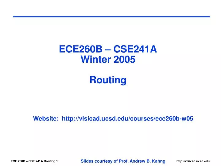
ECE260B – CSE241A Winter 2005 Routing. Website: http://vlsicad.ucsd.edu/courses/ece260b-w05. Slides courtesy of Prof. Andrew B. Kahng. Routing Region Definition. Placement Improvement. Global Routing. Cost Estimation. Routing Region Ordering. Routing Improvement. Detailed Routing.

E N D
ECE260B – CSE241AWinter 2005Routing Website: http://vlsicad.ucsd.edu/courses/ece260b-w05 Slides courtesy of Prof. Andrew B. Kahng
Routing Region Definition Placement Improvement Global Routing Cost Estimation Routing Region Ordering Routing Improvement Detailed Routing Cost Estimation Physical Design Flow Input Read Netlist Floorplanning Floorplanning Initial Placement Placement Routing Compaction/clean-up Output Write Layout Database
Routing Applications Mixed Cell and Block Cell-based Block-based
Standard Cell Layout Courtesy K. Keutzer et al. UCB
Routing Algorithms • Global routing • Guide the detailed router in large design • May perform quick initial detail routing • Commonly used in cell-based design, chip assembly, and datapath • Also used in floorplanning and placement • Detail routing • Connect all pins in each net • Must understand most or all design rules • May use a compactor to optimize result • Necessary in all applications Courtesy K. Keutzer et al. UCB
Routers Global Detailed Specialized Graph Search Power & Ground Restricted General Purpose Steiner Clock River Maze Iterative Switchbox Line Probe Channel Line Expansion Hierarchical Greedy Left-Edge Taxonomy of VLSI Routers Courtesy K. Keutzer et al. UCB
Global Routing • Objectives • Minimize wire length • Balance congestion • Timing driven • Noise driven • Keep buses together • Frameworks • Steiner trees • Channel-based routing • Maze routing
Global Routing Formulation • Given(i) Placement of blocks/cells • (ii) channel capacities • Determine • Routing topology of each net • Optimize • (i) max # nets routed • (ii) min routing area • (iii) min total wirelength Classic terminology: In general cell design or standard cell design, we are able to move blocks or cell rows, so we can guarantee connections of all the nets (“variable-die” + channel routers). Classic terminology: In gate-array design, exceeding channel capacity is not allowed (“fixed-die” + area routers). Since Tangent’s Tancell (~1986), and > 3LM processes, we use area routers for cell-based layout Courtesy K. Keutzer et al. UCB
Global Routing • Provide guidance to detailed routing (why?) • Objective function is application-dependent Courtesy K. Keutzer et al. UCB
Graph Models for Global Routing • Global routing problem is a graph problem • Model routing regions, their adjacencies and capacities as graph vertices, edges and weights • Choice of model depends on algorithm • Grid graph model • Grid graph represents layout as a hXw array, vertices are layout cells, edges capture cell adjacencies, zero-capacity edges represent blocked cells • Channel intersection graph model for block-based design Courtesy K. Keutzer et al. UCB
Global Routing Approaches • Can route nets: • Sequentially, e.g. one at a time • Concurrently, e.g. simultaneously all nets • Sequential approaches • Sensitive to ordering • Usually sequenced by • Criticality • Number of terminals • Concurrent approaches • Computationally hard • Hierarchical methods used Courtesy K. Keutzer et al. UCB
Sequential Approaches • Solve a single net routing problem • Differ depending on whether net is two- or multi-terminal • Two-terminal algorithms • Maze routing algorithms • Line probing • Shortest-path based algorithms • Multi-terminal algorithms • Steiner tree algorithms Courtesy K. Keutzer et al. UCB
Two-Terminal Routing: Maze Routing • Maze routing finds a path between source (s) and target (t) in a planar graph • Grid graph model is used to represent block placement • Available routing areas are unblocked vertices, obstacles are blocked vertices • Finds an optimal path • Time and space complexity O(hXw) Courtesy K. Keutzer et al. UCB
4 3 2 3 4 5 6 7 8 9 10 11 3 2 1 2 3 4 5 6 7 8 9 10 2 1 A 1 5 6 7 8 3 2 1 2 6 7 8 9 10 11 12 4 3 2 3 12 13 5 4 3 4 14 B 13 14 6 5 13 14 14 7 6 7 11 12 13 14 8 7 8 9 10 11 12 13 14 9 8 9 10 11 12 13 14 Maze Routing • Point to point routing of nets • Route from source to sink • Basic idea = wave propagation (Lee, 1961) • Breadth-first search + back-tracing after finding shortest path • Guarantees to find the shortest path • Objective = route all nets according to some cost function that minimizes congestion, route length, coupling, etc. Courtesy K. Keutzer et al. UCB
Maze Routing • Initialize priority queue Q, source S and sink T • Place S in Q • Get lowest cost point X from Q, put neighbors of X in Q • Repeat last step until lowest-cost point X is equal to the sink T • Rip and reroute nets, i.e., select a number of nets based on a cost function (e.g., congestion of regions through which net travels), then remove the net and reroute it • Main objective: reduce overflow • Edge overflow = 0 if num_nets less than or equal to the capacity • Edge overflow = num_nets – capacity if num_nets is greater than capacity • Overflow = Σ (edge overflows) over all edges Courtesy K. Keutzer et al. UCB
Maze Routing Cost Function and Directed Search • Points can be popped from queue according to a multivariable cost function • Cost = function(overflow,coupling,wire length, … ) • Add <distance to sink> to cost function directed search • Allows maze router to explore points around the direct path from source to sink first
Limiting the Search Region • Since majority of nets are routed within the bounding box defined by S and T, can limit points searched by maze router to those within bounding box • Allows maze router to finish sooner with little or no negative impact on final routing cost • Router will not consider points that are unlikely to be on the route path
Problems With Maze Routing Slow: for each net, we have to search NN grid Memory: total layout grid needs to be kept NxN Improvements • Simple speed-up • Minimum detour algorithm (Hadlock, 1977) • Fast maze algorithm (Soukup, 1978) • depth-first search until obstacle • breadth-first at obstacle • until target is reached • Will find a path if it exists, may be suboptimal • Typical speed-up 10-50x • Further improvements • Maze routing infeasible for large chips • Line search (Mikami & Tabuchi, 1968; Hightower, 1969) • Pattern routing Courtesy K. Keutzer et al. UCB
Line-Probe Algorithm • Mikami&Tabuchi IFIPS Proc, Vol H47, pp 1475-1478, 1968 • Mikami+Tabuchi’s algorithm • Generate search lines from both source and target (level-0 lines) • From every point on the level-i search lines, generate perpendicular level-(i+1) search lines • Proceed until a search line from the source meets a search line from a target • Will find the path if it exists, but not guaranteed to find the shortest path Time and space complexity: O(L), where Lis the number of line segments Courtesy K. Keutzer et al. UCB
Intersection of escape line Escape line Source probe Escape line Target probe Line-Probe Summary • Fast, handles large nets / distances / designs • Routing may be incomplete
Pattern-Based Routing • Restrict routing of net to certain basic templates • Basic templates are L-shaped (1 bend) or Z-shaped (2 bends) routes between a source and sink • Templates allow fast routing of nets since only certain edges and points are considered Courtesy K. Keutzer et al. UCB
A B D 4 C E Connecting Multi-Terminal Nets In general, maze and line-probe routing are not well-suited to multi-terminal nets Several attempts made to extend to multi-terminal nets • Connect one terminal at a time • Use the entire connected subtrees as sources or targets during expansion • Ripup/Reroute to improve solution quality (remove a segment and re-connect) 1 A 2 D 3 B C E • Results are sub-optimal • Inherit time and memory cost of maze and line-probe algorithms Courtesy K. Keutzer et al. UCB
Multi-terminal Nets: Different Routing Options (b) Steiner Tree with Trunk (15) (a) Steiner Tree (14) (d) Chain (17) (c) Minimum Spanning Tree (16) (e) Complete Graph (42) Cost is determined by routing model Courtesy K. Keutzer et al. UCB
Steiner Tree Based Algorithms • Tree interconnecting a set of points (demand points, D) and some other (intermediate) points (Steiner points, S) • If S is empty, Steiner Minimum Tree (SMT) equivalent to Minimum Spanning Tree (MST) • Finding SMT is NP-complete; many good heuristics • SMT typically 88% of MST cost; best heuristics are within ½ % of optimal on average • Underlying Grid Graph defined by intersection of horizontal and vertical lines through demand points (Hanan grid) Rectilinear SMT and MST problems • Can modify MST to approximate RMST, e.g., build MST and rectilinearize each edge
Minimum Spanning Tree (Prim’s construction) Given a weighted graph Find a spanning tree whose weight is minimum • Prim’s algorithm • start with an arbitrary node s • T{s} • while T is not a spanning tree • find the closest pair xV-T, yT • add (x,y) to T 8 6 7 9 x 8 4 g 5 7 2 2 4 5 s 10 3 5 10 runs in O(n2) time very simple to implement always gives a tree of minimum cost Courtesy K. Keutzer et al. UCB
Applying Spanning and Steiner Tree Algorithms • General cell/block design: channel intersection graphs • Standard-cell or gate-array design: RSMT or RMST in geometry or grid-graph Courtesy K. Keutzer et al. UCB
Problems with Sequential Routing Algorithms Net ordering • Must route net by net, but difficult to determine best net ordering! • Difficult to predict/avoid congestion • What can be done • Use other routers • Channel/switchbox routers • Hierarchical routers • Rip-up and reroute Courtesy K. Keutzer et al. UCB
Global Routing: Concurrent Approaches • Can formulate routing problem as integer programming, solve simultaneously for all nets Given (i) Set of Steiner trees for each net (ii) Placement of blocks/cells (iii) Channel capacities Determine Select a Steiner tree for each net w/o violating channel capacities Optimize Min total wirelength Courtesy K. Keutzer et al. UCB
Routers Global Detailed Specialized Graph Search Power & Ground Restricted General Purpose Steiner Clock River Maze Iterative Switchbox Line Probe Channel Line Expansion Hierarchical Greedy Left-Edge Taxonomy of VLSI Routers X { gridded, gridless} Courtesy K. Keutzer et al. UCB
P2 T1 P1 T2 One Layer Routing: General River-Routing • For clock, power, ground still may need to solve single-layer routing • Two possible paths per net along boundary • Path = alternating sequence of horizontal and vertical segments connecting two terminals of a net • Consider starting terminals and ending terminals • Assume every path counter-clockwise around boundary Courtesy K. Keutzer et al. UCB
One Layer Routing: General River-Routing • Create circular list of all terminals ordered counterclockwise according to position on boundary 4e 5e 6e 7e 8e 2e 8s 1s 7s 6s 1e 2s 3s 4s 3e 5s Courtesy K. Keutzer et al. UCB
4e 5e 6e 7e 8e 2e 8s 1s 7s 6s 1e 2s 3s 4s 3e 5s One Layer Routing: General River-Routing • Boundary-packed solution • Flip corners to minimize wire length Courtesy K. Keutzer et al. UCB
Routers Global Detailed Specialized Graph Search Power & Ground Restricted General Purpose Steiner Clock River Maze Iterative Switchbox Line Probe Channel Line Expansion Hierarchical Greedy Left-Edge Taxonomy of VLSI Routers Courtesy K. Keutzer et al. UCB
Channel vs. Switchbox • Channel may have exits at left and right sides, but exit positions are not fixed • We may map exits to either lower or upper edge of a channel • One dimensional problem • Terminal positions on all four sides of a switchbox are fixed • Two dimensional problem • Switchbox routing is more difficult 2 1 2 3 3 4 4 1 1 3 2 4 4 3 1 2 1 2 2 3 3 1 Courtesy K. Keutzer et al. UCB
Channel Routing Problem • Input: Pins on the lower and upper edge • Output: Connection of each net • Constraints (Assumption) • (i) grid structure • (ii) two routing layers. One for horizontal wires, the other for vertical wires • (iii) vias for connecting wires in two layers • Minimize: • (i) # tracks (channel height) • (ii) total wire length • (iii) # vias Courtesy K. Keutzer et al. UCB
net 1 1 branch via end tracks trunk 1 channel pins Channel Routing • Basic Terminology: • Fixed pin positions on top and bottom edges • Classical channel: no nets leave channel • Three-sided channel possible Courtesy K. Keutzer et al. UCB
Horizontal Constraint Graph (HCG) Node vi: represents a horizontal interval spanned by net i There is an edge between vi and vj if horizontal intervals overlap No two nets with a horizontal constraint may be assigned to the same track Maximum clique of HCG establishes lower bound on # of tracks: # tracks size of maximum clique of HCG a a a f e b c d a ld(x) a f b e c d Local density at column C, ld(C) = # nets split by column C Channel Density d = max ld(C) over all C Each net spans over an interval Horizontal Constraint Graph(HCG) is an undirected graph with: • vertex : net • edge: <n_j, n_k>, if intervals I_j, I_k intersect Courtesy K. Keutzer et al. UCB
Vertical Constraint Graph (VCG) a b b • Node: represents a net • Edge (a1a2) exists if at some column: • Net a1 has a terminal on the upper edge • Net a2 has a terminal on the lower edge • Edge a1a2 means that Net a1 must be above Net a2 • Establishes lower bound: # tracks longest path in VCG • VCG may have a cycle ! a b c c a b c a b a b a b Courtesy K. Keutzer et al. UCB
Doglegs in Channel Routing Doglegs may reduce the longest path in VCG a b c a b c c-2 c-1 a b c d d a b c d d a b c d a b c-1 c-2 d Doglegs break cycles in VCG b a b a b-1 a ? b-1 a b b-2 b-2 a b a b Courtesy K. Keutzer et al. UCB
1 1 4 10 2 3 5 7 9 4 5 6 6 3 8 8 7 2 10 9 Characterizing the Channel Routing Problem 0 1 4 5 1 6 7 0 4 9 10 10 4 10 1 7 6 5 9 2 3 8 2 3 5 3 5 2 6 8 9 8 7 9 Vertical constraint graph Gv Horizontal constraint graph Channel routing problem is completely characterized by the vertical constraint graph and the horizontal constraint graph. Courtesy K. Keutzer et al. UCB
Interval Packing • Theorem A set of intervals with density d can be packed into d tracks. • Proof: I1=(a,b) I2=(c,d) • Define: I1<I2 iff b<c or I1=I2 • reflexive: I1<I1 • anti-symmetric: I1<I2, I2<I1 I1=I2 • transitive: I1<I2, I2<I3I1<I3 Set of intervals with binary relation < forms a partially ordered set (POSET) • Intervals in a single track form a chain • Intervals intersecting a common column form an antichain • Dilworth’s theorem (1950): If the maximum antichain of a POSET is of size d, then the POSET can be partitioned into d chains I6 I5 I4 I3 I2 I1 a b c d I5 I2 I6 I4 I1 I3 Courtesy K. Keutzer et al. UCB
Left-Edge Algorithm for Interval Packing • Repeat • create a new track t • Repeat • put leftmost feasible interval to t • untilno more feasible interval • untilno more interval Intervals are sorted according to their left endpoints I6 I6 I5 I1 I5 I4 I3 I4 I2 I3 I1 I2 O(nlogn) time algorithm.Greedy algorithm works! Courtesy K. Keutzer et al. UCB
Routing completion Width and spacing rule Minimum width and spacing Variable width and spacing Connection Net Class of nets Tapering Poly M1 M2 Tapering Detailed Routing Objectives M1
Detailed Routing Objectives • Width and spacing rule Minimum spacing 0.4m >=2m >=2m >=2m 0.6m 0.8m Width-based Spacing
Detailed Routing Objectives • Via selection • Via array based on wire size or resistance • Rectangular via rotation and offset No rotation for a “cross” via Rotate and offset horizontal vias
simple pin Strong Weak Must complex pin Detailed Routing Objectives • Understand complex pin & equivalent pin modeling
Noisy region Extra space Grounded Shields Quiet region Segregation Spacing Shielding Detailed Routing Objectives • Noise-driven
Power Signal Ground M2 M1 Signal Poly Same-Layer Shielding Adjacent-Layer Shielding Detailed Routing Objective • Shielding • Same-layer shielding • Adjacent-layer shielding
Shield Bus Shielding Bus Detailed Routing Objective • Shielding • Bus shielding • Bus interleaving
Differential Detailed Routing Objectives • Differential pair routing • Balanced length or capacitance Balanced length