Download
1 / 55
590 likes | 945 Views
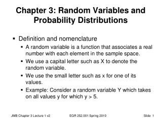
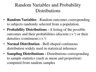
PROBABILITY (6MTCOAE205). Chapter 4 Continuous Random Variables and Probability Distributions. Probability Distributions. Probability Distributions. Ch. 3. Discrete Probability Distributions. Continuous Probability Distributions. Ch. 4. Binomial. Uniform. Hypergeometric. Normal.

E N D
PROBABILITY (6MTCOAE205) Chapter 4 Continuous Random Variables and Probability Distributions
Probability Distributions Probability Distributions Ch. 3 Discrete Probability Distributions Continuous Probability Distributions Ch. 4 Binomial Uniform Hypergeometric Normal Poisson Exponential
Continuous Probability Distributions • A continuous random variable is a variable that can assume any value in an interval • thickness of an item • time required to complete a task • temperature of a solution • height, in inches • These can potentially take on any value, depending only on the ability to measure accurately.
Cumulative Distribution Function • The cumulative distribution function, F(x), for a continuous random variable X expresses the probability that X does not exceed the value of x • Let a and b be two possible values of X, with a < b. The probability that X lies between a and b is
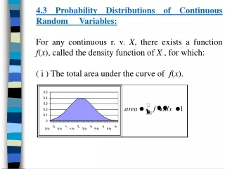
Probability Density Function The probability density function, f(x), of random variable X has the following properties: • f(x) > 0 for all values of x • The area under the probability density function f(x) over all values of the random variable X is equal to 1.0 • The probability that X lies between two values is the area under the density function graph between the two values
Probability Density Function (continued) The probability density function, f(x), of random variable X has the following properties: • The cumulative density function F(x0) is the area under the probability density function f(x) from the minimum x value up to x0 where xmis the minimum value of the random variable x
Probability as an Area Shaded area under the curve is the probability that X is between a and b f(x) ) ≤ ≤ P ( a x b ) < < = P ( a x b (Note that the probability of any individual value is zero) x a b
The Uniform Distribution Probability Distributions Continuous Probability Distributions Uniform Normal Exponential
The Uniform Distribution • The uniform distribution is a probability distribution that has equal probabilities for all possible outcomes of the random variable f(x) Total area under the uniform probability density function is 1.0 x xmin xmax
The Uniform Distribution (continued) The Continuous Uniform Distribution: f(x) = where f(x) = value of the density function at any x value a = minimum value of x b = maximum value of x
Properties of the Uniform Distribution • The mean of a uniform distribution is • The variance is
Uniform Distribution Example Example: Uniform probability distribution over the range 2 ≤ x ≤ 6: 1 f(x) = = .25 for 2 ≤ x ≤ 6 6 - 2 f(x) .25 x 2 6
Expectations for Continuous Random Variables • The mean of X, denoted μX , is defined as the expected value of X • The variance of X, denoted σX2 , is defined as the expectation of the squared deviation, (X - μX)2, of a random variable from its mean
Linear Functions of Variables • Let W = a + bX , where X has mean μX and variance σX2 , and a and b are constants • Then the mean of W is • the variance is • the standard deviation of W is
Linear Functions of Variables (continued) • An important special case of the previous results is the standardized random variable • which has a mean 0 and variance 1
The Normal Distribution Probability Distributions Continuous Probability Distributions Uniform Normal Exponential
The Normal Distribution (continued) • ‘Bell Shaped’ • Symmetrical • Mean, Median and Mode are Equal Location is determined by the mean, μ Spread is determined by the standard deviation, σ The random variable has an infinite theoretical range: + to f(x) σ x μ Mean = Median = Mode
The Normal Distribution (continued) • The normal distribution closely approximates the probability distributions of a wide range of random variables • Distributions of sample means approach a normal distribution given a “large” sample size • Computations of probabilities are direct and elegant • The normal probability distribution has led to good business decisions for a number of applications
Many Normal Distributions By varying the parameters μ and σ, we obtain different normal distributions
The Normal Distribution Shape f(x) Changingμ shifts the distribution left or right. Changing σ increases or decreases the spread. σ μ x Given the mean μand variance σwe define the normal distribution using the notation
The Normal Probability Density Function • The formula for the normal probability density function is Where e = the mathematical constant approximated by 2.71828 π = the mathematical constant approximated by 3.14159 μ = the population mean σ = the population standard deviation x = any value of the continuous variable, < x <
Cumulative Normal Distribution • For a normal random variable X with mean μ and variance σ2 , i.e., X~N(μ,σ2), the cumulative distribution function is f(x) x x0 0
Finding Normal Probabilities The probability for a range of values is measured by the area under the curve x a μ b
Finding Normal Probabilities (continued) x a μ b x a μ b x a μ b
The Standardized Normal Any normal distribution (with any mean and variance combination) can be transformed into the standardized normaldistribution (Z), with mean 0 and variance 1 Need to transform X units into Z units by subtracting the mean of X and dividing by its standard deviation f(Z) 1 Z 0
Example If X is distributed normally with mean of 100 and standard deviation of 50, the Z value for X = 200is This says that X = 200 is two standard deviations (2 increments of 50 units) above the mean of 100.
Comparing X and Z units 100 200 X (μ = 100, σ = 50) 0 2.0 Z ( μ = 0 , σ = 1) Note that the distribution is the same, only the scale has changed. We can express the problem in original units (X) or in standardized units (Z)
Finding Normal Probabilities f(x) x a b µ Z 0
Probability as Area Under the Curve The total area under the curve is 1.0, and the curve is symmetric, so half is above the mean, half is below f(X) 0.5 0.5 μ X
Appendix Table 1 • The Standardized Normal table shows values of the cumulative normal distribution function • For a given Z-value a , the table shows F(a) (the area under the curve from negative infinity to a ) Z a 0
The Standardized Normal Table • The Standardized Normal Tablegives the probability F(a) for any value a .9772 Example: P(Z < 2.00) = .9772 Z 0 2.00
The Standardized Normal Table (continued) • For negative Z-values, use the fact that the distribution is symmetric to find the needed probability: .9772 .0228 Example: P(Z < -2.00) = 1 – 0.9772 = 0.0228 Z 0 2.00 .9772 .0228 Z -2.00 0
General Procedure for Finding Probabilities • Draw the normal curve for the problem in terms of X • Translate X-values to Z-values • Use the Cumulative Normal Table To find P(a < X < b) when X is distributed normally:
Finding Normal Probabilities • Suppose X is normal with mean 8.0 and standard deviation 5.0 • Find P(X < 8.6) X 8.0 8.6
Suppose X is normal with mean 8.0 and standard deviation 5.0. Find P(X < 8.6) Finding Normal Probabilities (continued) μ = 8 σ = 10 μ= 0 σ = 1 X Z 8 8.6 0 0.12 P(X < 8.6) P(Z < 0.12)
Solution: Finding P(Z < 0.12) Standardized Normal Probability Table (Portion) P(X < 8.6) = P(Z < 0.12) z F(z) F(0.12) = 0.5478 .10 .5398 .11 .5438 .12 .5478 Z 0.00 .13 .5517 0.12
Upper Tail Probabilities • Suppose X is normal with mean 8.0 and standard deviation 5.0. • Now Find P(X > 8.6) X 8.0 8.6
Upper Tail Probabilities (continued) • Now Find P(X > 8.6)… P(X > 8.6) = P(Z > 0.12) = 1.0 - P(Z ≤ 0.12) = 1.0 - 0.5478 = 0.4522 0.5478 1.000 1.0 - 0.5478 = 0.4522 Z Z 0 0 0.12 0.12
Finding the X value for a Known Probability • Steps to find the X value for a known probability: 1. Find the Z value for the known probability 2. Convert to X units using the formula:
Finding the X value for a Known Probability (continued) Example: • Suppose X is normal with mean 8.0 and standard deviation 5.0. • Now find the X value so that only 20% of all values are below this X .2000 X ? 8.0 Z ? 0
Find the Z value for 20% in the Lower Tail 1. Find the Z value for the known probability • 20% area in the lower tail is consistent with a Z value of -0.84 Standardized Normal Probability Table (Portion) z F(z) .82 .7939 .80 .20 .83 .7967 .84 .7995 X ? 8.0 .85 .8023 Z -0.84 0
Finding the X value 2. Convert to X units using the formula: So 20% of the values from a distribution with mean 8.0 and standard deviation 5.0 are less than 3.80
Assessing Normality • Not all continuous random variables are normally distributed • It is important to evaluate how well the data is approximated by a normal distribution
The Normal Probability Plot • Normal probability plot • Arrange data from low to high values • Find cumulative normal probabilities for all values • Examine a plot of the observed values vs. cumulative probabilities (with the cumulative normal probability on the vertical axis and the observed data values on the horizontal axis) • Evaluate the plot for evidence of linearity
The Normal Probability Plot (continued) A normal probability plot for data from a normal distribution will be approximately linear: 100 Percent 0 Data
The Normal Probability Plot (continued) Left-Skewed Right-Skewed 100 100 Percent Percent 0 0 Data Data Uniform Nonlinear plots indicate a deviation from normality 100 Percent 0 Data
Normal Distribution Approximation for Binomial Distribution 5.4 • Recall the binomial distribution: • n independent trials • probability of success on any given trial = P • Random variable X: • Xi =1 if the ith trial is “success” • Xi =0 if the ith trial is “failure”
The shape of the binomial distribution is approximately normal if n is large The normal is a good approximation to the binomial when nP(1 – P) > 5 Standardize to Z from a binomial distribution: Normal Distribution Approximation for Binomial Distribution (continued)
Let X be the number of successes from n independent trials, each with probability of success P. If nP(1 - P) > 5, Normal Distribution Approximation for Binomial Distribution (continued)
40% of all voters support ballot proposition A. What is the probability that between 76 and 80 voters indicate support in a sample of n = 200 ? E(X) = µ = nP = 200(0.40) = 80 Var(X) = σ2 = nP(1 – P) = 200(0.40)(1 – 0.40) = 48 ( note: nP(1 – P) = 48 > 5 ) Binomial Approximation Example