Download
1 / 1
20 likes | 133 Views
Influence Function Approach to Sensitiveness of Kurtosis Indexes. Francesco Campobasso, Dipartimento di Scienze Statistiche Carlo Cecchi, Università degli Studi di Bari, Italy, e-mail: fracampo@dss.uniba.it. Introduction.

E N D
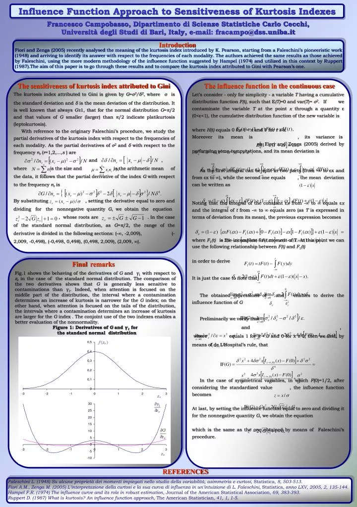
Influence Function Approach to Sensitiveness of Kurtosis Indexes Francesco Campobasso, Dipartimento di Scienze Statistiche Carlo Cecchi, Università degli Studi di Bari, Italy, e-mail: fracampo@dss.uniba.it Introduction Fiori and Zenga (2005) recently analysed the meaning of the kurtosis index introduced by K. Pearson, starting from a Faleschini’s pioneeristic work (1948) and arriving to identify its answer with respect to the frequencies of each modality. The authors achieved the same results as those achieved by Faleschini, using the more modern methodology of the influence function suggested by Hampel (1974) and utilized in this context by Ruppert (1987).The aim of this paper is to go through these results and to compare the kurtosis index attributed to Gini with Pearson’s one. The kurtosis index attributed to Gini is given by G=σ2/δ2, whereσis the standard deviation and δ is the mean deviation of the distribution. It is well known that always G≥1, that for the normal distribution G=π/2 and that values of G smaller (larger) than π/2 indicate platikurtosis (leptokurtosis). With reference to the originary Faleschini’s procedure, we study the partial derivatives of the kurtosis index with respect to the frequencies of each modality. As the partial derivatives of σ2and δwith respect to the frequency nr(r=1,2,...,s ) are and , where is the size and is the arithmetic mean of the data, it follows that the partial derivative of the index G with respect to the frequency nr is By substituting , setting the derivative equal to zero and dividing for the nonnegative quantity G, we obtain the equation , whose roots are . In the case of the standard normal distribution, as G=π/2, the range of the derivative is divided in the following sections: (-∞, -2,009), (-2,009, -0,498), (-0,498, 0,498), (0,498, 2,009), (2,009, ∞). Let’s consider - only for simplicity - a variable T having a cumulative distribution function F(t), such that E(T)=0 and var(T)= σ2. If we contaminate the variable T at the point x through a quantity ε(0<ε<1), the cumulative distribution function of the new variable is where H(t) equals 0 for t < x and 1 for t ≥ x. Moreover its mean is , its variance is as Fiori and Zenga (2005) derived by performing some computations, and its mean deviation is As the first integral can be split in two parts (from -∞ to εx and from εx to ∞), while the second one equals , the mean deviation can be written as Noting that the integral of the constant εx from -∞ to ∞ equals εx and the integral of t from -∞ to ∞ equals zero (as T is expressed in terms of deviation from its mean), the previous expression becomes where F1(t)is the incomplete first moment of T. At this point we can use the following relationship between F(t) and F1(t) in order to derive It is just the case to note that The obtained expressions of and enables to derive the influence function of G Preliminarily we verify that and , where equals 1 for x < 0 and 0 for x ≥ 0; then we find, by means of de L’Hospital’s rule, that In the case of symmetrical variables, in which F(0)=1/2, after considering the standardized value , the influence function becomes At last, by setting the influence function equal to zero and dividing it for the nonnegative quantity G, we obtain the equation which is the same as the one obtained by means of Faleschini’s procedure. The influence function in the continuous case The sensitiveness of kurtosis index attributed to Gini Finalremarks Fig.1 shows the behaving of the derivatives of G and γ1with respect to zr in the case of the standard normal distribution. The comparison of the two derivatives shows that G is generally less sensitive to contaminations than γ1. Indeed, when attention is focused on the middle part of the distribution, the interval where a contamination determines an increase of kurtosis is narrower for the G index; on the other hand, when attention is focused on the tails of the distribution, the intervals where a contamination determines an increase of kurtosis are larger for the G index . The conjoint use of the two indexes enables a better evaluation of the nonnormality. Figure 1: Derivatives of G and γ1 for the standard normal distribution REFERENCES FaleschiniL. (1948) Su alcune proprietà dei momenti impiegati nello studio della variabilità, asimmetria e curtosi, Statistica, 8, 503-513. Fiori A.M., Zenga M. (2005) L’interpretazione della curtosi e la sua curva di influenza in un’intuizione di L. Faleschini, Statistica, anno LXV, 2005, 2, 135-144. Hampel F.R. (1974) The influence curve and its role in robust estimation, Journal of the American Statistical Association, 69, 383-393. Ruppert D. (1987) What is kurtosis? An influence function approach, The American Statistician, 41, 1, 1-5.