Download
1 / 24
270 likes | 548 Views
Valuation 10: Hedonic Pricing. A partial equilibrium model of prices, wages and pollution The hedonic price equation From hedonic prices to welfare Application: Environmental hazards. Last two weeks we looked at.

E N D
Valuation 10: Hedonic Pricing • A partial equilibrium model of prices, wages and pollution • The hedonic price equation • From hedonic prices to welfare • Application: Environmental hazards
Last two weeks we looked at • The household production function approach, which assumes that certain observable behaviour is a complement (e.g., travel to recreate) or substitute (e.g., airbag for road safety) to unobservable consumption of an environmental good or service • A simple travel cost model of a single site • Multiple sites • Implementation • The zonal travel cost method • The individual travel cost model • Travel cost with a random utility model
The price of land • The asset price equals the value of the stream of services that the parcel can be expected to provide in the future, netted back to the present • uncertainty about the future • The rental price of land is the value of renting for a short period • e.g., for agricultural land, the difference between expected yield times prices minus the costs of labour, seeds, pesticides etc • expectations about the future play little or no role • Pollution degrades value and thus price • What is the WTP to clean up the pollution?
Starters • What is the WTP to clean up pollution? • Consider agricultural land in a valley, half of which is upwind a polluting plant, the other half downwind • If this is a small valley with a local market for agricultural goods the land value change will not fully capture the value for cleaner air • If this is a small valley in a large market the difference between land value is a proxy of the value of pollution • Consider an open city, with free mobility • Utility must be the same everywhere • So land prices exactly compensate for pollution • In a closed city, reducing non-uniform pollution would affect property values as well as utility
Wages, land prices and pollution • Arguably, pollution should suppress land prices – but we see that urban land is worth more than rural land • Urban wages are also higher than rural wages – do wages rise to compensate for deteriorating environmental quality? • We will construct a model of urban land prices, wages and pollution -- first, analytically and then we‘ll derive a function that can be estimated
The consumer • Consider a number of cities that have different levels of pollution p; firms produce a composite good X (at price 1) and move about freely; the wage rate w and the land rent r vary between cities • Consumers are identical, purchase X and land for housing L • Each consumer has the utility maximization problem: • The utility level for a particular set of w, r and p is • Assuming free movement, utility is the same everywhere
The producer • In a constant cost industry, the average cost of producing X equals the product price which is the same for all cities • The price for the product is the same, but the composition of inputs can differ • If rents are higher in one city, wages must be lower to compensate, otherwise the firm would relocate • Pollution may affect costs in different ways • Unproductive (pollution hinders production) • Productive (pollution regulation hinders production) • Neutral (no affect on the firm, but wages and rents affect production)
Productive and unproductive pollution Two cities with different pollution levels: p2> p1 • Cases A and B: when pollution is productive wages rise • Cases C and D: when pollution is unproductive land prices decrease r c(w,r,p2)=1 c(w,r,p1)=1 V(w,r,p1)=k V(w,r,p2)=k C A B D w
Sum up • Because the utility levels of the citizens must be the same, higher pollution must be compensated by either higher wages, lower land rents or both • If pollution is productive, the firm spends less on pollution control • To keep costs constant for higher levels of pollution, wages or land prices must rise • Putting consumers and producers together • If pollution is productive, pollution raises wages but has an ambiguous effect on land rents • If pollution is unproductive, pollution depresses land prices but has an ambiguous effect on wages • If pollution is neutral, pollution decreases land prices and increases wages
Hedonic price theory • In the “real world” we are often confronted with bundles of goods with a single price for the whole bundle • We are interested in the price of an element of the bundle • This is the focus of the hedonic price theory • By observing the prices of many houses with different characteristics, we can infer the implicit value that is being placed on one characteristic, e.g. air quality • By observing wages associated with many different occupations we can infer the value of small changes in e.g. risk • Applied to prices of farmland as early as 1922 • Rosen (1974) developed the formal theory of hedonic prices
Hedonic price theory (2) • Consider an homogenous area that can be considered a single market from the point of view of, say, houses • For simplification, each house is characterised by a single characteristic, z, say, air pollution • We are interested in the relation between price and air quality, p = p(z) • The price function is an equilibrium concept (partial equilibrium) resulting from interaction of supply and demand • We assume that the market is perfect • Both producers and consumers take p(z) as given
The consumer • The consumer buys one house as well as other goods x • The consumer’s problem is: • What is the amount of x for particular values of z to achieve a certain level of utility: • The budget for buying the house, guaranteeing a certain level of utility is • Alternatively, we can define the consumer’s problem as • This is known as the bid function – it tells you the maximum amount a consumer is willing to pay as a function of income and air pollution
Consumer choice • Hedonic price function and two bid functions for two different levels of utility $ p(z) Q(y,z,U0) Q(y,z,U1) Utility increases Air quality z
The producer • The costs c of producing one house depend on input prices r and the characteristics z: c(r,z) • The producer maximises profits • Alternatively the price to obtain a certain level of profit given a level of z is • This is known as the offer function – it tells you the minimum amount a producer is willing to accept as a function of costs and air pollution
Producer choice • Hedonic price function and two offer functions for two different levels of profit $ F(r,z, p2) Profits increase F(r,z, p1) p(z) Air quality z
Market equilibrium In the equilibrium, the marginal bid, the marginal offer, and the house price are identical – all parties in the market value the house the same, at the margin p(z) $ F3 Q3 F2 Q2 F1 Q1 Air quality z
Willingness to pay $/unit Marginal implicit price function and marginal WTP for one more unit of z for consumers 1 and 2 MWTP2(z) MWTP1(z) p‘(z) Air quality z
Sum up • The hedonic price function tells you how price varies with environmental quality and other factors (income) • Take the derivative of the rental price to environmental quality – this gives the price of environmental quality • This is the first-stage estimation procedure • Do this for various income levels • This gives the price of environmental quality as a function of income – that is, an inverse demand function • This is the second-stage estimation procedure • This assumes, that different individuals making choices along the hedonic price function are variants of the same person • As the second-stage estimation procedure uses no additional data beyond the already contained in the hedonic price function, it can only reproduce the coefficients estimated from the hedonic price function • Recent applications of the method estimate only the first-stage
Theory and practice • Theory and practice differ substantially • Niceties such as the difference between compensated and uncompensated demand functions are typically ignored • Critical assumptions: • Households have full information on all housing prices and attributes, transaction and moving costs are zero • Prices adjust instantaneously to changes • Market distortions are ignored • Only one market (housing) is analysed • The reason: data; although wages and house prices are known, it is hard to get data because of privacy
Application: Environmental hazards • Do environmental hazards such as the proximity to a major fuel pipeline affect house prices? • Study by Hansen, Benson and Hagen (Land Economics, 2006) • They use data for Bellingham, Washington, • the site of a 1999 rupture and explosion and compare housing prices before and after the accident (1995-2004) • The results suggest that the event led to a significant increase in perceived risk and perhaps to an increase beyond the actual risk • Before the accident public awareness was low and risks were irrelevant indicating a deviation between perceived and actual risk
Data and modelling strategy • In Bellingham, two major transmission pipelines run through residential area • The Olympic pipeline (refined petroleum) and the Trans Mountain pipeline (crude oil) • On June 10, 1999, the Olympic pipeline ruptured, spilling 229000 gallons of gasoline into the Whatcom Creek • Sales of all houses located within one mile of either pipeline was sampled for the period 1995 to 2004 • A number of housing characteristics were included as well as the distance to a pipeline • To test the hypothesis (sales price are not affected in the absence of an effect) they split the sample to estimate the model for each sub-sample, the pre-event and the post-event sample
Regression results * Significant at the 1% level; ** significant at the 5% level; *** significant at the 10% level.
As distance increases, sales price rises to the average level
The effect decays over time, but a significant price effect remains