Edge Relaxation

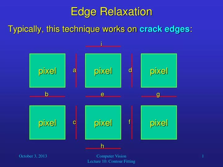
1. f d a c i g h e b Edge Relaxation • Typically, this technique works on crack edges: pixel pixel pixel pixel pixel pixel Computer Vision Lecture 10: Contour Fitting

2. Edge Relaxation • Edges h and i can be used for non-maxima suppression similar to the Canny detector. We will not discuss this here. • The edge pattern at an edge e can be described as a pair of integers: the number of connecting edges on the left (edges a, b, c) and the number of connecting edges on the right (d, f, g). • Since the left and right sides are exchangeable, we simply write the smaller number first, e.g. 0-1, 1-3, 2-2. • These edge patterns determine whether we should increase or decrease the current confidence value for e or leave it unchanged. Computer Vision Lecture 10: Contour Fitting

3. Edge Relaxation • These are the actions we should take: • 0-0: isolated edge – decrease edge confidence • 0-1: uncertain – increase slightly or leave unchanged • 0-2, 0-3: dead end – decrease • 1-1: continuation: increase strongly • 1-2, 1-3: continuation to border intersection: increase • 2-2, 2-3, 3-3: bridge between borders – no change Computer Vision Lecture 10: Contour Fitting

4. Edge Relaxation • Now we can describe the edge relaxation algorithm: • Evaluate a confidence c(1)(e) for all crack edges e in the image. • Find the edge type of each edge based on edge confidences c(k)(e) in its neighborhood. • Update the confidence c(k+1)(e) of each edge e according to its type and its previous confidence c(k)(e). • Stop if all edge confidences have converged either to 0 or 1. Repeat steps (2) and (3) otherwise. Computer Vision Lecture 10: Contour Fitting

5. Edge Relaxation • At the start of the algorithm, we can determine c(1)(e) for all crack edges e as the normalized (between 0 and 1) edge strength yielded by the edge detector. • Often local normalization works better, because it limits the influence of individual, extremely high edge strengths. • Since during the iterations we often have edge confidence values between 0 and 1, how can we determine edge types? • In order to determine the edge pattern and the edge type, we can simply use confidence thresholds. • Another method is shown on the next slide. Computer Vision Lecture 10: Contour Fitting

6. Edge Relaxation • Consider the three adjacent edges on one side of e. • Let’s call them a, b, and c so that a  b  c. • Let’s further define a value q (something like a threshold); usually q = 0.1. • Finally, let’s define m = max(a, b, c, q) • Then the edge type on that side is defined as k, where type(k) is the maximum of the following numbers: • type(0) = (m – a)(m – b)(m – c) • type(1) = a(m – b)(m – c) • type(2) = ab(m – c) • type(3) = abc Computer Vision Lecture 10: Contour Fitting

7. Edge Relaxation • Based on the edge type we decide whether we want to increase or decrease the confidence for e (or leave it unchanged). • This can be done as follows: • Increase: c(k+1)(e) = min(1, c(k)(e) + ) • Decrease: c(k+1)(e) = max(0, c(k)(e) - ) • Appropriate values for  are typically in the range between 0.1 and 0.3. Computer Vision Lecture 10: Contour Fitting

8. Edge Relaxation • After a large number of iterations, it is possible that the results of edge relaxation deteriorate. • A possible solution is to use an upper threshold T1 and a lower threshold T2 and use them as follows: • If c(k+1)(e) > T1 then assign c(k+1)(e) = 1, • If c(k+1)(e) < T2 then assign c(k+1)(e) = 0. Computer Vision Lecture 10: Contour Fitting

9. Contours • Once we have a good idea of where our contours are, what is the best way to represent them? • A good contour representation should meet the following criteria: • Efficiency: The contour should be a simple, compact representation. • Accuracy: The contour should accurately fit the image features. • Effectiveness: The contour should be suitable for the operations to be performed in later stages of the application. Computer Vision Lecture 10: Contour Fitting

10. Contours • The accuracy of a contour representation is determined by • the form of the curve used to model the contour, • the performance of the curve-fitting algorithm, and • the accuracy of the estimation of edge locations. • Using an ordered list of edges as the representation is simple and as precise as the edge information itself. • It is not a compact representation and may be difficult to process in subsequent stages. Computer Vision Lecture 10: Contour Fitting

11. Contours • Using an appropriate curve model increases the accuracy of the representation. • This is because errors in the location of individual edges can be eliminated (if the correct model is used!). • The result is a more compact representation that is well-suited for subsequent analysis. • We will talk about • the elementary differential geometry of 2D curves, • techniques for calculating contour properties, and • curve models and how to fit them to contours. Computer Vision Lecture 10: Contour Fitting

12. Definitions • We will use the term edge to refer to edge points regardless of the edge orientation. • Most standard algorithms do not consider the orientation of edges, but just their location. • Definitions: • An edge list is an ordered set of edge points or fragments. • A contour is an edge list or the curve that has been used to represent the edge list. • A boundary is the closed contour that surrounds a region. Computer Vision Lecture 10: Contour Fitting

13. Geometry of Curves • We usually avoid the description of curves in the x-y plane by functions of the kind y = f(x). • This is because this notation only allows one y-value for a given x-value. • So, for example, it cannot be used to describe a circle, rectangle, or any other closed contour. • Instead, we will use the parametric form (x(u), y(u)). • It uses two functions x(u) and y(u) of a parameter u to specify the points along the curve from a starting point p1 = (x(u1), y(u1)) to an end point p2 = (x(u2), y(u2)). Computer Vision Lecture 10: Contour Fitting

14. Geometry of Curves • The length of the curve is given by the arc length: The unit tangent vector is given by: where p(u) = (x(u), y(u)) and p’(u) = (x’(u), y’(u)). Computer Vision Lecture 10: Contour Fitting

15. Geometry of Curves • Imagine three points along our curve:p(u + ), p(u), and p(u - ). • If these three points all differ from each other, then there is exactly one circle that passes through all three points. • In the limit   0, this circle is the osculating (touching) circle of the curve at the point u. • The center of this circle lies along the line containing the normal to the curve at point u. • The curvature is the inverse of the radius of the osculating circle. Computer Vision Lecture 10: Contour Fitting

16. Digital Curves • When we are dealing with actual curves in digital images, the situation is slightly different. • There are only eight possible angles between neighboring pixels, which makes the computation of slope and curvature difficult. • The idea to overcome this problem is to also account for non-adjacent edge points. • Let pn= (in, jn) be the coordinates of edge n in our edge list. • Then the k-slope is the (angle) direction vector between points that are k edges apart. Computer Vision Lecture 10: Contour Fitting

17. Geometry of Curves • The left k-slope is the direction from pn-kto pn, andthe right k-slope is the direction from pnto pn+k. • The k-curvature is the difference between the left and right k-slopes. • If we have N edge points (i1, j1) to (iN, jN) in the edge list, then we can approximate the length S of the digital curve as follows: Computer Vision Lecture 10: Contour Fitting