Download
1 / 92
930 likes | 1.08k Views
last updated on **March. 19, 2013 Matthew Valenti **and Terry Ferrett Iterative Solutions and West Virginia University Morgantown, WV 26506-6109 mvalenti@wvu.edu. A Guided Tour of CML, the Coded Modulation Library. Outline. CML overview What is it? How to set it up and get started?

E N D
last updated on **March. 19, 2013 Matthew Valenti **and Terry Ferrett Iterative Solutions and West Virginia University Morgantown, WV 26506-6109 mvalenti@wvu.edu A Guided Tour of CML,the Coded Modulation Library
CML Overview Outline CML overview What is it? How to set it up and get started? Uncoded modulation Simulate uncoded BPSK and QAM in AWGN and Rayleigh fading Coded modulation Simulate a turbo code from UMTS 25.212 Ergodic (Shannon) capacity analysis Determine the modulation constrained capacity of BPSK and QAM Outage analysis Determine the outage probability over block fading channels. Determine the outage probability of finite-length codes The internals of CML Throughput calculation Convert BLER to throughput for hybrid-ARQ
CML Overview What is CML? CML is an open source toolbox for simulating capacity approaching codes in Matlab. Available for free at the Iterative Solutions website: www.iterativesolutions.com Runs in matlab, but uses c-mex for efficiency. First release was in Oct. 2005. Used code that has been developed starting in 1996.
CML Overview Features Simulation of BICM (bit interleaved coded modulation) Turbo, LDPC, or convolutional codes. PSK, QAM, FSK modulation. BICM-ID: Iterative demodulation and decoding. Generation of ergodic capacity curves BICM/CM constrained modulation. Information outage probability Block fading channels. Blocklength-constrained channels (AWGN or fading) Calculation of throughput of hybrid-ARQ.
CML Overview Supported Standards Binary turbo codes: UMTS/3GPP, including HSDPA and LTE. cdma2000/3GPP2. CCSDS. Duobinary turbo codes: DVB-RCS. WiMAX IEEE 802.16. LDPC codes: DVB-S2. Mobile WiMAX IEEE 802.16e.
CML Overview Simulation Data is Valuable CML saves simulation state frequently parameter called “save_rate” can be tuned to desired value. CML can be stopped at any time. Intentionally: Hit CTRL-C within matlab. Unintentionally: Power failure, reboot, etc. CML automatically resumes simulation If a simulation is run again, it will pickup where it left off. Can reset simulation by setting “reset=1”. SNR points can be added or deleted prior to restarting. Simulations can be made more confident by requesting additional trials prior to restarting. The new results will be added to the old ones.
CML Overview Compiled Mode A flag called “compiled_mode” can be used to run CML independently of matlab. CML must first be compiled using the matlab compiler. Advantages: Can run on machines without matlab. Can run on a grid computer.
CML Overview WebCML WebCML is a new initiative sponsored by NASA and NSF. Idea is to upload simulation parameters to a website and hit a “simulate” button. Simulation begins on the webserver. The webserver will divide the simulation into multiple jobs which are sent to a grid computer. Results can be retrieved while simulation is running and once it has completed. The grid is comprised of ordinary desktop computers. The grid compute engine is a screen saver. Kicks in only when computer is idle. Users of WebCML are encouraged to donate their organizations computers to the grid.
CML Overview Getting Started with CML Download www.iterativesolutions.com/download.htm Unzip into a directory Root directory will be ./cml About simulation databases A large database of previous simulation results can be downloaded. Unzip each database and place each extracted directory into the ./cml/output directory About c-mex files. C-mex files are compiled for PC computers. For unix and mac computers, must compile. Within matlab, cd to ./cml/source and type “make”.
CML Overview Starting and Interacting with CML Launch matlab Cd to the ./cml directory Type “CmlStartup” This sets up paths and determines the version of matlab. To run CML, only two functions are needed: CmlSimulate Runs one or more simulations. Simulation parameters are stored in text files. Currently .m scripts, to be changed to XML files soon. The argument tells CML which simulation(s) to run. CmlPlot Plots the results of one or more simulations.
CML Overview Scenario Files and the SimParam Structure The parameters associated with a set of simulations is stored in a scenario file. Located in one of two directories ./cml/scenarios for publicly available scenarios ./cml/localscenarios for personal user scenarios Other directories could be used if they are on the matlab path. .m extension. Exercise Edit the example scenario file: UncodedScenarios.m The main content of the scenario file is a structure called sim_param Sim_param is an array. Each element of the array is called a record and corresponds to a single distinct simulation.
CML Overview Common Parameters List of all parameters can be found in: ./cml/mat/DefineStructures.m ./cml/documentation/readme.pdf Default values are in the DefineStructures.m file Some parameters can be changed between runs, others cannot. sim_param_changeable sim_param_unchangeable
CML Overview Dissecting the SimParam Structure:The simulation type sim_param(record).sim_type = ‘uncoded’ BER and SER of uncoded modulation ‘coded’ BER and FER of coded modulation ‘capacity’ The Shannon capacity under modulation constraints. ‘outage’ The information outage probability of block fading channels Assumes codewords are infinite in length ‘bloutage’ Information outage probability in AWGN or ergodic/block fading channels Takes into account lenth of the code. ‘throughput’ By using FER curves, determines throughput of hybrid ARQ This is an example of an analysis function … no simulation involved.
CML Overview Lesser Used Simulation Types sim_param(record).sim_type = ‘bwcapacity’ Shannon capacity of CPFSK under bandwidth constraints. ‘minSNRvsB’ Capacity limit of CPFSK as a function of bandwidth
CML Overview Parameters Common to All Simulations Sim_param(record). comment = {string} Text, can be anything. legend = {string} What to put in figure caption linetype = {string} Color, type, and marker of line. Uses syntax from matlab “plot”. filename = {string} Where to save the results of the simulation Once filename is changed, any parameter can be changed. reset = {0,1} with default of 0 Indication to resume “0” or restart “1” simulation when run again. If reset = 1, any parameter may be changed.
CML Overview Specifying the Simulation sim_param(record). SNR = {vector} Vector containing SNR points in dB Can add or remove SNR points between runs SNR_type = {‘Eb/No in dB’ or ‘Es/No in dB’} For some simulation types, only one option is supported. E.g. for capacity simulations, it must be Es/No save_rate = {scalar integer} An integer specifying how often the state of the simulation is saved Number of trials between saves. Simulation echoes a period ‘.’ every time it saves.
CML Overview Specifying the Simulation (cont’d) sim_param(record). max_trials = {vector} A vector of integers, one for each SNR point Tells simulation maximum number of trials to run per point. max_frame_errors = {vector} Also a vector of integers, one for each SNR point. Tells simulation maximum number of frame errors to log per point. Simulation echoes a ‘x’ every time it logs a frame error. minBER = {scalar} Simulation halts once this BER is reached minFER = {scalar} Simulation halts once this FER is reached.
CML Overview Outline CML overview What is it? How to set it up and get started? Uncoded modulation Simulate uncoded BPSK and QAM in AWGN and Rayleigh fading Coded modulation Simulate a turbo code from UMTS 25.212 Ergodic (Shannon) capacity analysis Determine the modulation constrained capacity of BPSK and QAM Outage analysis Determine the outage probability over block fading channels. Determine the outage probability of finite-length codes The internals of CML Throughput calculation Convert BLER to throughput for hybrid-ARQ
CML Overview Specifying Modulation sim_param(record). modulation = {string} Specifies the modulation type May be ‘BPSK’, ‘QPSK’, ‘QAM’, ‘PSK’, ‘APSK’, ‘HEX’, or ‘FSK’ ‘HSDPA’ used to indicate QPSK and QAM used in HSDPA. All but FSK are 2 dimensional modulations Uses a complex scalar value for each symbol. Default is ‘BPSK’ New (version 1.9 and above): Can also be set to “custom”. mod_order = {integer scalar} Number of points in the constellation. Power of 2. Default is 2. In some cases, M=0 is used to indicate an unconstrained Gaussian input. S_matrix = {complex vector} Only used for “custom” modulation type. A vector of length “mod_order” containing the values of the symbols in the signal set S.
CML Overview Specifying Modulation sim_param(record). mapping = {integer vector} A vector of length M specifying how data bits are mapped to symbols. Vector contains the integers 0 through M-1 exactly once. ith element of vector is the set of bits associated with the ith symbol. Alternatively, can be a string describing the modulation, like ‘gray’ or ‘sp’ Default is ‘gray’ framesize = {integer scalar} The number of symbols per Monte Carlo trial For coded systems, this is number of bits per codeword demod_type = {integer scalar} A flag indicating how to implement the demodulator 0 = log-MAP (approximated linearly) 1 = max-log-MAP 2 = constant-log-MAP 3 and 4 other implementations of log-MAP Max-log-MAP is fastest. Does not effect the uncoded error rate. However, effects coded performance
CML Overview M-ary Complex Modulation = log2 M bits are mapped to the symbol xk, which is chosen from the set S = {x1, x2, …, xM} The symbol is multidimensional. 2-D Examples: QPSK, M-PSK, QAM, APSK, HEX These 2-D signals take on complex values. M-D Example: FSK FSK signals are represented by the M-dimensional complex vector X. The signaly = hxk + n is received h is a complex fading coefficient (scalar valued). n is complex-valued AWGN noise sample More generally (FSK), Y = h X + N Flat-fading: All FSK tones multiplied by the same fading coefficient h. Modulation implementation in CML The complex signal set S is created with the CreateConstellation function. Modulation is performed using the Modulate function.
CML Overview Log-likelihood of Received Symbols Let p(xk|y) denote the probability that signal xkS was transmitted given that y was received. Let f(xk|y) = p(xk|y), where is any multiplicative term that is constant for all xk. When all symbols are equally likely, f(xk|y) f(y|xk) For each signal in S, the receiver computes f(y|xk) This function depends on the modulation, channel, and receiver. Implemented by the Demod2D and DemodFSK functions, which actually computes log f(y|xk). Assuming that all symbols are equally likely, the most likely symbol xk is found by making a hard decision on f(y|xk) or log f(y|xk).
CML Overview Example: QAM over AWGN. Let y = x + n, where n is complex i.i.d. N(0,N0/2 ) and the average energy per symbol is E[|x|2] = Es
CML Overview Converting symbol liklihoods to bit LLR The symbol likelihoods must be transformed into bit log-likelihood ratios (LLRs): where represents the set of symbols whose nth bit is a 1. and is the set of symbols whose nth bit is a 0. log f(Y|Xk) Modulator: Pick Xk S Receiver: Compute log f(Y|Xk)for every Xk S Xk Y Demapper: Compute n from set of log f(Y|Xk) data n to decoder Nk SoMAP function Demod2D function 000 001 100 101 011 010 111 110
CML Overview Log-domain Implementation log-MAP demod_type = 0 max-log-MAP demod_type = 1
The max* function 0.7 0.6 0.5 0.4 0.3 fc(|y-x|) 0.2 0.1 0 -0.1 0 1 2 3 4 5 6 7 8 9 10 |y-x|
CML Overview FSK-Specific Parameters sim_param(record). h = {scalar} The modulation index h=1 is orthogonal csi_flag = {integer scalar} 0 = coherent (only available when h=1) 1 = noncoherent w/ perfect amplitudes 2 = noncoherent without amplitude estimates
CML Overview Specifying the Channel sim_param(record). channel = {‘AWGN’, ‘Rayleigh’, ‘block’} ‘Rayleigh’ is “fully-interleaved” Rayleigh fading ‘block’ is for coded simulation type only blocks_per_frame = {scalar integer} For block channel only. Number of independent blocks per frame. Block length is framesize/blocks_per_frame bicm = {integer scalar} 0 do not interleave bits prior to modulation 1 interleave bits prior to modulation (default) 2 interleave and perform iterative demodulation/decoding This option is irrelevant unless a channel code is used
CML Overview Exercises Create and run the following simulations: BPSK in AWGN 64QAM with gray labeling in AWGN 64QAM with gray labeling in Rayleigh fading Choices that need to be made? Framesize? Save_rate? Min_BER? Min_frame_errors? Demod_type? Plot all the results on the same figure.
CML Overview Outline CML overview What is it? How to set it up and get started? Uncoded modulation Simulate uncoded BPSK and QAM in AWGN and Rayleigh fading Coded modulation Simulate a turbo code from UMTS 25.212 Ergodic (Shannon) capacity analysis Determine the modulation constrained capacity of BPSK and QAM Outage analysis Determine the outage probability over block fading channels. Determine the outage probability of finite-length codes The internals of CML Throughput calculation Convert BLER to throughput for hybrid-ARQ
CML Overview Coded Systems:Code Configuration Only for sim_param(record).sim_type = ‘coded’ sim_param(record).code_configuration = {scalar int} 0 = Convolutional 1 = binary turbo code (PCCC) 2 = LDPC 3 = HSDPA turbo code 4 = UMTS turbo code with rate matching 5 = WiMAX duobinary tailbiting turbo code (CTC) 6 = DVB-RCS duobinary tailbiting turbo code
CML Overview Convolutional Codes Only rate 1/n mother codes supported. Can puncture to higher rate. Code is always terminated by a tail. Can puncture out the tail. sim_param(record). g1 = {binary matrix} Example: (133,171) code from Proakis g1 = [1 0 1 1 0 1 1 1 1 1 1 0 0 1]; Constraint length = number of columns Rate 1/n where n is number of rows. nsc_flag1 = {scalar integer} 0 for RSC 1 for NSC Can handle cyclic block codes as a rate 1 terminated RSC code
CML Overview Convolutional Codes: Decoding Algorithms sim_param(record).decoder_type = {integer scalar} negative value for Viterbi algorithm 0 = log-MAP (approximated linearly) 1 = max-log-MAP 2 = constant-log-MAP 3 and 4 other implementations of log-MAP Decodes over entire trellis (no sliding window traceback)
CML Overview Punctured Convolutional Codes sim_param(record). pun_pattern1 = {binary matrix} Puncturing pattern n rows arbitrary number of columns (depends on puncture period) 1 means keep bit, 0 puncture it. number greater than 1 is number of times to repeat bit. tail_pattern1 = {binary matrix} tail can have its own puncturing pattern.
CML Overview Turbo Codes sim_param(record). Parameters for first constituent code g1 nsc_flag1 pun_pattern1 tail_pattern1 Parameters for second constituent code g2 nsc_flag2 pun_pattern2 tail_pattern2
CML Overview Turbo Codes (cont’d) sim_param(record). code_interleaver = {string} A string containing the command used to generate the interleaver. Examples include: “CreateUmtsInterleaver(5114)” % UMTS interleaver. “CreateLTEInterleaver(6144)” % LTS interleaver. “CreateCCSDSInterleaver(8920)” % CCSDS interleaver. “randperm(40)-1” % a random interleaver of length 40. Can replace above lengths with other valid lengths. decoder_type = {integer scalar} Same options as for convolutional codes (except no Viterbi allowed). max_iterations = {integer scalar} Number of decoder iterations. Decoder will automatically halt once codeword is correct. plot_iterations = {integer scalar} Which iterations to plot, in addition to max_iterations
CML Overview UMTS Rate Matching sim_param(record) framesize = {integer scalar} number of data bits code_bits_per_frame = {integer scalar} number of code bits When code_configuration = 4, automatically determines rate matching parameters according to UMTS (25.212)
CML Overview HSDPA Specific Parameters sim_param(record). N_IR = {integer scalar} Size of the virtual IR buffer X_set = {integer vector} Sequence of redundancy versions (one value per ARQ transmission) P = {integer scalar} Number of physical channels per turbo codeword Examples from HSET-6 TS 25.101 N_IR = 9600 QPSK framesize = 6438 X_set = [0 2 5 6] P = 5 (i.e. 10 physical channels used for 2 turbo codewords) 16-QAM framesze = 9377 X_set = [6 2 1 5] P = 4 (i.e. 8 physical channels used for 2 turbo codewords)
CML Overview LDPC sim_parameters(record). parity_check_matrix = {string} A string used to generate the parity check matrix decoder_type 0 Sum-product (default) 1 Min-sum 2 Approximate-min-star max_iterations Number of decoder iterations. Decoder will automatically halt once codeword is correct. plot_iterations Which iterations to plot, in addition to max_iterations
CML Overview Block Fading For coded simulations, block fading is supported. Sim_param(record).channel = ‘block’ Sim_param(record).blocks_per_frame The number of independent blocks per frame Example, HSDPA with independent retransmissions blocks_per_frame = length(X_set );
CML Overview Exercises Simulate A convolutional code with g=(7,5) over AWGN with BPSK The same convolutional code punctured to rate 3/4. The UMTS turbo code with 16-QAM Unpunctured w/ 640 input bits Punctured to force the rate to be 1/2. Compare log-MAP and max-log-MAP HSDPA HSET-6 Quasi-static block fading
CML Overview Outline CML overview What is it? How to set it up and get started? Uncoded modulation Simulate uncoded BPSK and QAM in AWGN and Rayleigh fading Coded modulation Simulate a turbo code from UMTS 25.212 Ergodic (Shannon) capacity analysis Determine the modulation constrained capacity of BPSK and QAM Outage analysis Determine the outage probability over block fading channels. Determine the outage probability of finite-length codes The internals of CML Throughput calculation Convert BLER to throughput for hybrid-ARQ
CML Overview Noisy Channel Coding Theorem(Shannon 1948) Consider a memoryless channel with input X and output Y The channel is completely characterized by p(x,y) The capacity C of the channel is where I(X,Y) is the (average) mutual information between X and Y. The channel capacity is an upper bound on information rate r. There exists a code of rate r < C that achieves reliable communications. “Reliable” means an arbitrarily small error probability. X Y Source p(x) Channel p(y|x) Receiver
CML Overview Capacity of the AWGN Channel with Unconstrained Input Consider the one-dimensional AWGN channel The capacity is The X that attains capacity is Gaussian distributed. Strictly speaking, Gaussian X is not practical. The input X is drawn from any distribution with average energy E[X2] = Es X Y = X+N N~zero-mean white Gaussian with energy E[N2]= N0/2 bits per channel use
CML Overview Capacity of the AWGN Channel with a Modulation-Constrained Input Suppose X is drawn with equal probability from the finite set S = {X1,X2, …, XM} where f(Y|Xk) = p(Y|Xk) for any common to all Xk Since p(x) is now fixed i.e. calculating capacity boils down to calculating mutual info. Modulator: Pick Xk at random from S= {X1,X2, …, XM} ML Receiver: Compute f(Y|Xk) for every Xk S Xk Y Nk
CML Overview Entropy and Conditional Entropy Mutual information can be expressed as: Where the entropy of X is And the conditional entropy of X given Y is where self-information where
CML Overview Calculating Modulation-Constrained Capacity To calculate: We first need to compute H(X) Next, we need to compute H(X|Y)=E[h(X|Y)] This is the “hard” part. In some cases, it can be done through numerical integration. Instead, let’s use Monte Carlo simulation to compute it.
CML Overview Step 1: Obtain p(x|y) from f(y|x) Since We can get p(x|y) from Modulator: Pick Xk at random from S Receiver: Compute f(Y|Xk) for every Xk S Xk Y Nk Noise Generator
CML Overview Step 2: Calculate h(x|y) Given a value of x and y (from the simulation) compute Then compute Modulator: Pick Xk at random from S Receiver: Compute f(Y|Xk) for every Xk S Xk Y Nk Noise Generator
CML Overview Step 3: Calculating H(X|Y) Since: Because the simulation is ergodic, H(X|Y) can be found by taking the sample mean: where (X(n),Y(n)) is the nth realization of the random pair (X,Y). i.e. the result of the nth simulation trial. Modulator: Pick Xk at random from S Receiver: Compute f(Y|Xk) for every Xk S Xk Y Nk Noise Generator