Download
1 / 35
350 likes | 471 Views
Atmospheres of Cool Stars. Radiative Equilibrium Models Extended Atmospheres Heating Theories. Radiative Equilibrium Models. Gustafson et al. (2005): MARCS code difficult because of UV “line haze” (millions of b-b transitions of Fe I in 300-400 nm range, and Fe II in 200-300 nm range)

E N D
Atmospheres of Cool Stars Radiative Equilibrium ModelsExtended AtmospheresHeating Theories
Radiative Equilibrium Models • Gustafson et al. (2005): MARCS codedifficult because of UV “line haze”(millions of b-b transitions of Fe I in 300-400 nm range, and Fe II in 200-300 nm range) • Convection important at depth • Metallicity and line blanketing causes surface cooling and back warming
Dwarfs Giants • Solid line = Solar abundances[Fe/H]=0 • Dashed line =Metal poor[Fe/H]=-2 • Dot-dashed =Kurucz LTE-RE model
Semi-empirical Models Based on Observations of Iλ(μ=1,τ=1) • Solar spectrum shows non-thermal components at very long and short wavelengths that indicate importance of other energy transport mechanisms
Determine central specific intensity across spectrum • Get brightness temperaturefrom Planck curve for Iλ • From opacity get optical depth on standard depth scale • T(h) for h=height
Reality: Structured and Heated Optical:photosphere EUV: higher X-ray: higher yet
Photosphere Chromosphere Transition region Corona Wind Extended Atmospheres
Corona • Observed during solar eclipses or by coronagraph (electron scattering in optical) • Nearly symmetric at sunspot maximum, equatorially elongated at sunspot minimum • Structure seen in X-rays (no X-ray emission from cooler, lower layers) • Coronal lines identified by Grotrian, Edlén (1939): Fe XIV 5303, Fe X 6374, Ca XV 5694 • High ionization level and X-rays indicate T~106 K
Chromosphere • Named for bright colors (“flash spectrum”) observed just before and after total eclipse • H Balmer, Fe II, Cr II, Si II lines present: indicates T = 6000 – 10000 K • Lines from chromosphere appear in UV (em. for λ<1700 Å; absorption for λ>1700 Å) • Large continuous opacity in UV, but lines have even higher opacity: appear in emission when temperature increases with height
Transition Region • Seen in high energy transitions which generally require large energies (usually in lines with λ<2000 Å) • Examples in solar spectrum:Si IV 1400, C IV 1550 (resonance or ground state transitions)
Stellar Observations • Chromospheric and transition region lines seen in UV spectra of many F, G, K-type stars (International Ultraviolet Explorer) • O I 1304, C I 1657, Mg II 2800 • Ca II 3968, 3933 (H, K) lines observed as emission in center of broad absorption (related to sunspot number in Sun; useful for starspots and rotation in other stars) • Emission declines with age (~rotation)
Chromospheres in H-R Diagram • Emission lines appear in stars found cooler than Cepheid instability strip • Red edge of strip formed by onset of significant convection that dampens pulsations • Suggests heating is related to mechanical motions in convection
Coronae in H-R Diagram • Upper luminosity limit for stars with transition region lines and X-ray coronal emission • Heating not effective in supergiants (but mass loss seen)
Theory of Atmospheric Heating • Increase in temperature cannot be due to radiative or thermal processes • Need heating by mechanical or magneto-electrical processes
Acoustic Heating • Large turbulent velocities in solar granulation are sources of acoustic (sound) waves • Lightman (1951), Proudman (1952) show that energy flux associated with waves iswhere v = turbulent velocity and cs = speed of sound
Acoustic Heating • Acoustic waves travel upwards with energy flux = (energy density) x (propagation speed)= ½ ρv2cs • If they do not lose energy, then speed must increase as density decreases→ form shock waves that transfer energy into the surrounding gas
Wave Heating • In presence of magnetic fields, sound and shock waves are modified into magneto-hydrodynamic (MHD) waves of different kinds • Damping (energy loss) of acoustic modes depends on wave period:ex. 5 minute oscillations of Sun in chromosphere with T = 10000 K yields a damping length of λ = 1500 km
Wave Heating • Change in shock flux with height is • Energy deposited (dissipated into heat) at height h is where
Wave Heating • Energy also injected by Alfvén waves (through Joule heating caused by current through a resistive medium) • Observations show spatial correlation between sites of enhanced chromospheric emission and magnetic flux tube structures emerging from surface: magnetic processes cause much of energy dissipation
Balance Heating and Cooling • Energy loss by radiation through H b-f recombination in Lyman continuum (λ < 912 Å) and collisional excitation of H • In chromosphere, H mainly ionized, primary source of electrons • for H recombination for H collisional excitation • Similar relations exist for other ions
Radiative Loss Function • Below T = 15000 K, f(T) is a steep function of T because of increasing H ionization • Above T = 15000 K, H mostly ionized so it no longer contributes much to cooling • He ionization becomes a cooling source for T > 20000 K: • Above T=105 K, most abundant species are totally ionized → slow decline in f(T)
Energy Balance • In lower transition region (hot) Pg = 2 PeElectron density:Radiation loss rate:(almost independent of T since f(T)~T2.0) • Set T(h) by Einput = Erad • Suppose Einput = Fmech(h) / λ
(1) Einput = constantT(h) increases with h Increasing height in outer atmosphere Each line down corresponds to a 12% drop in Pg or a 26% drop in Pg2
(2) Einput declines slowly with hT(h) still increases with h
(3) Einput declines quickly with hT(h) may not increase with h No T increase for damping lengthλ and pressure scale height H ifλ < H/2H is large in supergiants so heating in outer atmosphere does not occur.
Temperature Relation for Dwarfs • Suppose λ >> H in lower transition region so that Fmech(h) / λ ≈ constant Constant temperature gradient
Heating in the Outer Layers • T>105 K, rad. losses cannot match heating • T increases until loss by conductive flux downwards takes over (+ wind, rad. loss) • Conductive flux (from hot to cool regions by faster speeds of hotter particles) • Find T(h) from (η ~ 10-6 c.g.s.)