Download
1 / 41
460 likes | 756 Views
Convex Hulls in 3-space. (slides mostly by Jason C. Yang). Problem Statement. Given P : set of n points in 3D Return: Convex hull of P : CH ( P ) , i.e. smallest polyhedron s.t. all elements of P on or in the interior of CH ( P ). Complexity.

E N D
Convex Hullsin 3-space (slides mostly by Jason C. Yang) Lecture 10: Convex Hulls in 3D
Problem Statement • Given P: set of n points in 3D • Return: • Convex hull of P: CH(P), i.e. smallest polyhedron s.t. all elements of P on or inthe interior of CH(P). Lecture 10: Convex Hulls in 3D
Complexity • Complexity of CH for n points in 3D is O(n) • ..because the number of edges of a convex polytope with n vertices is at most 3n-6 and the number of facets is at most 2n-4 • ..because the graph defined by vertices and edges of a convex polytope is planar • Euler’s formula: n – ne + nf = 2 Lecture 10: Convex Hulls in 3D
Each face has at least 3 arcs Each arc incident to two faces 2ne 3nf Using Euler nf 2n-4ne 3n-6 Complexity Lecture 10: Convex Hulls in 3D
Algorithm • Randomized incremental algorithm • Steps: • Initialize the algorithm • Loop over remaining points Add pr to the convex hull of Pr-1to transform CH(Pr-1) to CH(Pr)[for integer r1, let Pr:={p1,…,pr} ] Lecture 10: Convex Hulls in 3D
Initialization • Need a CH to start with • Build a tetrahedron using 4 points in P • Start with two distinct points in P, say, p1 and p2 • Walk through P to find p3that does not lie on the line through p1and p2 • Find p4 that does not lie on the plane through p1, p2, p3 • Special case: No such points exist? Planar case! • Compute random permutation p5,…,pn of the remaining points Lecture 10: Convex Hulls in 3D
Inserting Points into CH • Add pr to the convex hull of Pr-1to transform CH(Pr-1) to CH(Pr) • Two Cases: • Pr is inside or on the boundary of CH(Pr-1) • Simple: CH(Pr) = CH(Pr-1) 2) Pr is outside of CH(Pr-1) – the hard case Lecture 10: Convex Hulls in 3D
Case 2: Pr outside CH(Pr-1) • Determine horizon of pr on CH(Pr-1) • Closed curve of edges enclosing the visible region of pr on CH(Pr-1) Lecture 10: Convex Hulls in 3D
Visibility • Consider plane hfcontaining a facetf of CH(Pr-1) • fis visible from a point p if that point lies in the open half-space on the other side of hf Lecture 10: Convex Hulls in 3D
Rethinking the Horizon • Boundary of polygon obtained from projecting CH(Pr-1) onto a plane with pr as the center of projection Lecture 10: Convex Hulls in 3D
CH(Pr-1) CH(Pr) • Remove visible facets from CH(Pr-1) • Found horizon: Closed curve of edges of CH(Pr-1) • Form CH(Pr) by connecting each horizon edge to pr to create a new triangular facet Lecture 10: Convex Hulls in 3D
Algorithm So Far… • Initialization • Form tetrahedron CH(P4) from 4 points in P • Compute random permutation of remaining pts. • For each remaining point in P • pr is point to be inserted • If pr is outside CH(Pr-1) then • Determine visible region • Find horizon and remove visible facets • Add new facets by connecting each horizon edge to pr How do we determine the visible region? Lecture 10: Convex Hulls in 3D
How to Find Visible Region • Naïve approach: • Test every facet with respect to pr • O(n2) work • Trick is to work ahead: Maintain information to aid in determining visible facets. Lecture 10: Convex Hulls in 3D
Conflict Lists • For each facet fmaintain Pconflict(f) {pr+1, …, pn} containing points to be inserted that can see f • For each pt, where t > r, maintain Fconflict(pt) containing facets of CH(Pr) visible from pt • p and fare in conflict because they cannot coexist on the same convex hull Lecture 10: Convex Hulls in 3D
Conflict Graph G • Bipartite graph • pts not yet inserted • facets on CH(Pr) • Arc for every point-facet conflict • Conflict sets for a point or facet can be returned in linear time At any step of our algorithm, we know all conflicts between the remaining points and facets on the current CH Lecture 10: Convex Hulls in 3D
G p5 f1 p6 f2 p7 Initializing G • Initialize G with CH(P4) in linear time • Walk through P5-n to determine which facet each point can see p6 f2 f1 p7 p5 Lecture 10: Convex Hulls in 3D
G G p5 p5 f1 f1 p6 p6 f2 f2 p7 p7 G p5 f1 f3 f3 p6 f2 p7 Updating G • Discard visible facets from pr by removing neighbors of pr in G • Remove pr from G • Determine new conflicts p6 f2 f1 p7 Lecture 10: Convex Hulls in 3D p5
pt Determining New Conflicts • If ptcan see newf, it can see edge e of f. • e on horizon of pr, so ewas already in and visible from pt in CH(Pr-1) • If pt seese, it saw eitherf1 or f2in CH(Pr-1) • Pt was in Pconflict(f1) or Pconflict(f2) in CH(Pr-1) Lecture 10: Convex Hulls in 3D
pt Determining New Conflicts • Conflict list of fcan be found by testing the points in the conflict lists of f1 and f2incident to the horizon edge e in CH(Pr-1) Lecture 10: Convex Hulls in 3D
Pconflict(f) for any funaffected by pr remains unchanged • Deleted facets not on horizon already accounted for pt What About the Other Facets? • Pconflict(f) for any f unaffected by pr remains unchanged Lecture 10: Convex Hulls in 3D
Final Algorithm • Initialize CH(P4) and G • For each remaining point • Determine visible facets for prby checking G • Remove Fconflict(pr) from CH • Find horizon and add new facets to CHand G • Update G for new facets by testing the points in existing conflict lists for facets in CH(Pr-1) incident to e on the new facets • Delete prand Fconflict(pr) from G Lecture 10: Convex Hulls in 3D
Fine Point • Coplanar facets • prlies in the plane of a face of CH(Pr-1) • fis not visible from prso we merge created triangles coplanar to f • New facet has same conflict list as existing facet Lecture 10: Convex Hulls in 3D
Analysis Lecture 10: Convex Hulls in 3D
Expected Number of Facets Created • Will show that expected number of facets created by our algorithm is at most 6n-20 • Initialized with a tetrahedron = 4 facets Lecture 10: Convex Hulls in 3D
Expected Number of New Facets • Backward analysis: • Remove pr from CH(Pr) • Number of facets removed same as those created by pr • Number of edges incident to pr in CH(Pr) is degree ofpr: deg(pr, CH(Pr)) Lecture 10: Convex Hulls in 3D
Expected Degree of pr • Convex polytope ofr vertices has at most 3r-6 edges • Sum of degrees of vertices of CH(Pr) is 6r-12 • Expected degree of pr bounded by (6r-12)/r Lecture 10: Convex Hulls in 3D
Expected Number of Created Facets • 4 from initial tetrahedron • Expected total number of facets created by adding p5,…,pn Lecture 10: Convex Hulls in 3D
Running Time • Initialization O(nlogn) • Creating and deleting facets O(n) • Expected number of facets created is O(n) • Deleting pr and facets in Fconflict(pr) from Galong with incident arcs O(n) • Finding new conflicts O(?) Lecture 10: Convex Hulls in 3D
Total Time to Find New Conflicts • For each edge e on horizon we spend O(|P(e|) time where P(e) =Pconfict(f1)Pconflict(f2) • Total time is O(eL |P(e)|) • Lemma 11.6The expected value of e|P(e)|, where the summation is over all horizon edges that appear at some stage of the algorithm is O(nlogn) Lecture 10: Convex Hulls in 3D
Randomized Insertion Order Lecture 10: Convex Hulls in 3D
Running Time • Initialization O(nlogn) • Creating and deleting facets O(n) • Updating G O(n) • Finding new conflicts O(nlogn) • Total Running Time is O(nlogn) Lecture 10: Convex Hulls in 3D
Convex Hulls in Dual Space • Upper convex hull of a set of points is essentially the lower envelope of a set of lines (similar with lower convex hull and upper envelope) Lecture 10: Convex Hulls in 3D
Half-Plane Intersection • Convex hulls and intersections of half planes are dual concepts • An algorithm to compute the intersection of half-planes can be given by dualizing a convex hull algorithm. Is this true? Lecture 10: Convex Hulls in 3D
Half-Plane Intersection • Duality transform cannot handle vertical lines • If we do not leave the Euclidean plane, there cannot be any general duality that turns the intersection of a set of half-planes into a convex hull. Why?Intersection of half-planes can be empty! And Convex hull is well defined. Conditions for duality: Intersection is not empty Point in the interior is known. • Duality transform cannot handle vertical lines • If we do not leave the Euclidean plane, there cannot be any general duality that turns the intersection of a set of half-planes into a convex hull. Why? Intersection of half-planes can be empty! And Convex hull is well defined. • Conditions for duality: • Intersection is not empty • Point in the interior is known. Lecture 10: Convex Hulls in 3D
Voronoi Diagrams Revisited • U:=(z=x2+y2) a paraboloid • p is point on plane z=0 • h(p) is non-vert planez=2pxx+2pyy-(p2x+p2y) • q is any point on z=0 • vdist(q',q(p)) = dist(p,q)2 • h(p) and paraboloid encodes any distance p to any point on z=0 Lecture 10: Convex Hulls in 3D
Voronoi Diagrams • H:={h(p) | p P} • UE(H) upper envelope of the planes inH • Projection of UE(H) on plane z=0 is Voronoi diagram of P Lecture 10: Convex Hulls in 3D
Simplified Case Lecture 10: Convex Hulls in 3D
Demo • http://www.cse.unsw.edu.au/~lambert/java/3d/delaunay.html Lecture 10: Convex Hulls in 3D
Delaunay Triangulations from CH Lecture 10: Convex Hulls in 3D
Higher Dimensional Convex Hulls • Upper Bound Theorem: The worst-case combinatorial complexity of the convex hull of n points in d-dimensional space is (n d/2). • Our algorithm generalizes to higher dimensions with expected running time of (nd/2) Lecture 10: Convex Hulls in 3D
Higher Dimensional Convex Hulls • Best known output-sensitive algorithm for computing convex hulls in Rd is: O(nlogk +(nk)1-1/(d/2+1)logO(n)) where k is complexity Lecture 10: Convex Hulls in 3D