Download
1 / 32
330 likes | 464 Views
Tuning and Validation of Ocean Mixed Layer Models. David Acreman. In partnership to provide world-class ocean forecasting and research. Overview. The FOAM system The ocean “mixed layer” Kraus-Turner and KPP models Model performance and tuning at OWS Papa

E N D
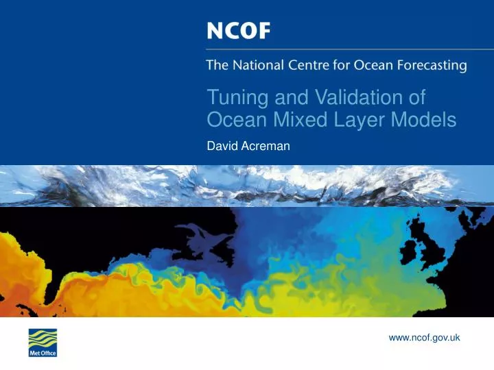
Tuning and Validation of Ocean Mixed Layer Models David Acreman
In partnership to provide world-class ocean forecasting and research
Overview • The FOAM system • The ocean “mixed layer” • Kraus-Turner and KPP models • Model performance and tuning at OWS Papa • Model performance and tuning vs Argo data • Effect of tuning in a global model
Forecasting the open ocean: the FOAM system Input boundary data NWP 6 hourly fluxes Obs QC Forecast to T+144 Analysis Output boundary data Real-time data Automatic verification Product delivery FOAM = Forecasting Ocean Assimilation Model • Operational real-time deep-ocean forecasting system • Daily analyses and forecasts out to 6 days • Low resolution global to high resolution nested configurations • Relocatable system deployable in a few weeks • Hindcast capability (back to 1997)
The Mixed Layer (1) • Surface layer of the ocean where temperature, salinity and density are near uniform due to turbulent mixing. • Mixed layer deepens due to wind mixing and convection. • Mixed layer shallows when winds are low and solar heating restores stratification. • The depth of the mixed layer shows seasonal variability (deepens in autumn, shallows in spring).
The Mixed Layer (2) • Mixed layer depth is an important output from FOAM • Properties of the mixed layer affect ocean-atmosphere fluxes. • Mixed layer depth also influences biological processes.
Mixed Layer Depth diagnostic Use the “Optimal mixed layer depth” definition of Kara et al. Search for a density difference which corresponds to a temperature difference of 0.8 C at the reference depth. Figure from Kara et al, 2000, JGR, 105 (C7), 16803
The Kraus-Turner Model • The Met Office ocean model uses a bulk mixed layer model, based on Kraus and Turner (1967), to mix tracers. • The model assumes a well mixed surface layer and uses a TKE budget to calculate mixed layer depth. • A 1D configuration was used to validate and tune the model.
K-Profile Parameterisation of Large et al • More sophisticated than KT. • Doesn’t assumed well mixed surface layer. • Models turbulent fluxes as diffusion terms. • Based on atmospheric boundary layer models.
Ocean Weather Station Papa • Frequently used for validation and tuning of 1D mixed layer models • Located in N.E. Pacific at 50N, 145W • Ran Kraus-Turner and KPP models for one year starting in March 1961 (same as Large et al 1994) • Used vertical resolutions of 0.5m, 2m, 5 and 10m • Forcing fluxes calculated using bulk formulae (met data courtesy of Paul Martin)
Tuning the Kraus-Turner Model • KT model based on a TKE budget. • Sources of TKE are wind mixing and convection. • Generation of TKE due to wind mixing given by W=u*3 • 15% of PE released by convection is converted to TKE. • TKE reduced by work done in overturning stable stratification and by dissipation. • Dissipation represented by exponential decay with depth: TKE~ exp (z/). • The free parameters and can be tuned to improve performance (currently =0.7, =100m in FOAM).
Tuning at OWS Papa • Ran many model realisations with different values of and parameters • Calculated mean and RMS errors in mixed layer depth • Plotted errors vs. and parameters • Tuned at 10m, 2m and 0.5m vertical resolutions
OWS Papa Tuning Results (10m resolution) Mean errors RMS errors Minimum RMS errors with =0.775, =40m
OWS Papa Tuning Results (2m resolution) Mean errors RMS errors Minimum RMS errors with =1.275, =30m
OWS Papa Tuning Results (0.5m resolution) Mean errors RMS errors Minimum RMS errors with =1.225, =30m
Temperature and temperature error from tuned OWS Papa K-T model
Model tuning using Argo data • Argo floats are autonomous profiling floats which record temperature and salinity profiles approximately every 10 days. • A large number of annual cycles are available for model tuning.
Kraus-Turner Model Tuning using Argo • Forcing from Met Office NWP fluxes. • Initial conditions from Levitus climatology. • Temperature and salinity profiles assimilated over 10 day window. • Vertical model levels based on operational FOAM system (~10m near surface). • Calculate mean and RMS errors, excluding cases with significant advection. • Average over sample of 218 floats. • Run KT model using different values of and .
Tuning results: all floats RMS errors Mean errors Smallest RMS errors with =1.5, =40m
Tuning results: assimilation of one profile only RMS errors Mean errors Smallest RMS errors with =1.1, =40m
Case study: Argo float Q4900131 • Location: 46N, 134W. • Forcing from Met Office NWP fluxes. • Initial conditions from float temperature and salinity profiles. • No assimilation of data. • Compare three different models: Kraus-Turner, Large and GOTM. • Run models at high vertical resolution (0.5m) and study annual cycle.
Case study: Argo float Q4900131 (2) • K-T model uses =0.7, =100m. • GOTM version 3.2 • GOTM results courtesy of Chris Jeffery (NOC).
Case study: Argo float Q4900131 (3) • KT model uses l=1.5, d=40m.
New parameters in global FOAM • Ran 1 year hindcast using global 1 degree FOAM • Kraus-Turner parameters were changed to =1.5, =40m • Plotted difference in mixed layer depth between models with old and new parameters
Conclusions • The Kraus-Turner model can give a good representation of mixed layer depths when tuned. • Optimum parameters for the Kraus-Turner scheme are =1.5, =40m with assimilation. • Without ongoing assimilation the optimum value of is reduced. • The Large et al KPP scheme tends to give mixed layers which are too shallow particularly at low vertical resolutions.