Download
1 / 43
430 likes | 547 Views
Data-driven dictionary definition for diverse document domains. Michael W. Mahoney Yahoo! Research http://www.cs.yale.edu/homes/mmahoney (Joint work with P. Drineas, S. Muthukrishnan and others as listed.). Modeling data and documents. People studying “documents,” or data more generally:

E N D
Data-driven dictionary definition for diverse document domains Michael W. Mahoney Yahoo! Research http://www.cs.yale.edu/homes/mmahoney (Joint work with P. Drineas, S. Muthukrishnan and others as listed.)
Modeling data and documents People studying “documents,” or data more generally: • put the data onto a graph or into a vector space • even if the data don’t naturally or obviously live there • and perform graph operations or vector space operations • to extract information from the data. Such data “documents” often have structure unrelated to the graphical or linear algebraic structure implicit in the modeling. • This non-modeled structure is difficult to formalize. Practitioners often have extensive field-specific intuition about the data. • This intuition is often used to choose “where the data live.” • The choice of where the data live may capture non-modeled structure.
Documents modeled as matrices Matrices often arise since n objects (“documents,” genomes, images, web pages), each with m features, may be represented by an m x n matrix A. Such “documents” often have structure: • for linear structure, SVD or PCA is often used, • for non-linear structure, kernel, e.g., diffusion-based, methods used, Note: We know what the rows/columns “mean” from the application area. Goal: Develop principled provably-accurate algorithmic methods such that: • they are agnostic with respect to any particular field, • one can fruitfully couple them to the field-specific intuition, • they perform well on complex non-toy data “documents”.
SVD of a matrix Theorem: Any m x n matrix A can be decomposed as: U (V): orthogonal matrix containing the left (right) singular vectors of A. S: diagonal matrix containing the singular values of A, ordered non-increasingly. : rank of A, the number of non-zero singular values. Data Application: Principal Components Analysis (PCA) is just SVD. Complexity: Exact computation of the SVD takes O(min{mn2 , m2n}) time.
SVD and low-rank approximations Theorem: Truncate the SVD by keeping k ≤ terms: • This gives another matrix Ak of the same dimensions that is the “best” approximation to A among all rank-k matrices. • Interesting property: For future reference, note: • The rows of Uk (= UA,k) are NOT orthogonal and are NOT unit length. • The lengths/Euclidean norms of the rows of Uk capture a notion of information dispersal.
Rows of left singular vectors What do the lengths of the rows of the n x d matrix U = UA “mean”? Consider possible n x d matrices U of d left singular vectors: In|k = k columns from the identity row lengths = 0 or 1 In|k x -> x Hn|k = k columns from the n x n Hadamard (real Fourier) matrix row lengths all equal Hn|k x -> maximally dispersed Uk = k columns from any orthogonal matrix row lengths between 0 and 1 The lengths of the rows of U = UA correspond to a notion of information dispersal
Problems with SVD/Eigen-Analysis Problems arise since structure in the data is not respected by mathematical operations on the data: • Reification - maximum variance directions are just that. • Interpretability - what does a linear combination of 6000 genes mean. • Sparsity - is destroyed by orthogonalization. • Non-negativity - is a convex and not linear algebraic notion. The SVD gives a low-rank matrix approximation with a very particular structure (think: rotation-with-truncation;rescaling;rotation-back-up). Question: Do there exist “better” low-rank matrix approximations. • “better” structural properties for certain applications. • “better” at respecting relevant structure. • “better” for interpretability and informing intuition.
Dictionaries for document analysis Discrete Fourier Transform (DCT): • fj = i=0,…,N-1 xn cos[j(n+1/2)/N] • the basis is fixed. • O(N2) or O(Nlog(N)) computation to determine coefficients. Singular Value Decomposition (SVD): • A = i=1,…, iU(i)V(i)T= i=1,…, i A[i] • O(N3) computation to determine basis and coefficients. Many other more complex/expensive procedures depending on the application. Question: Can actual data points and/or feature vectors be the dictionary. • “Core-sets” on graphs. • “CUR-decompositions” on matrices.
Dictionaries & the SVD A = U VT = i=1,..., iU(i)V(i)T, • where U(i),V(i) = eigen-cols and eigen-rows. Approximate: A(j)≈ i=1,...,k zijU(i) • by minzij|| A(j)- i=1,...,k zijU(i) ||2 Z = UkTA --> A ≈ Ak = (UkUkT)A • project onto space of top k eigen-cols. Z = kVkT --> A ≈ Ak = Uk(kVkT) • approximate every column of A i.t.o. a small number of eigen-rows and a low-dimensional encoding matrix k.
Dictionaries & columns and rows A = CUR = ij uijC(i)R(i), where U=W+ and W = intersection of C and R, • where C(i),R(i) = actual-cols and actual-rows. Approximate: A(j)≈ i=1,...,c yijC(i) • by minyij|| A(j)- i=1,...,c yijC(i) ||2 Y = C+A --> A ≈ PCA = (CC+)A • project onto space of those c actual-cols. Y ≈W+R --> A ≈ PCA ≈ C(W+R) • approximate every column of A i.t.o. a small number of actual-rows and a low-dimensional encoding matrix U=W+.
Carefully chosen U O(1) rows O(1) columns CX and CUR matrix decompositions Def: A CX matrix decomposition is a low-rank approximation explicitly expressed in terms of a small number of columns of the original matrix A. Def: A CUR matrix decomposition is a low-rank approximation explicitly expressed in terms of a small number of rows and columns of the original matrix A.
Problem formulation (1 of 3) Consider (for now) just columns: • Could ask to find the “best” k of n columns of A (by whatever measure-of-merit). • Combinatorial problem - trivial algorithm takes nk time. • Probably NP-hard if k is not fixed. Instead: • Fix a rank parameter k. • Let’s over-sample columns by a little (e.g., k+3, 10k, k2, etc.). • Get close (additive error or relative error) to the “best” rank-k approximation.. Note: Error and over-sampling are computational resources to exploit algorithmically.
Problem formulation (2 of 3) Ques: Do there exist O(k), or O(k2), or …, columns s.t.: ||A-CC+A||2,F < ||A-Ak||2,F + ||A||F Ans: Yes - and can find them in O(m+n) space and time after two passes over the data! (DFKVV99,DKM04) Ques: Do there exist O(k), or O(k2), or …, columns s.t.: ||A-CC+A||2,F < (1+)-1||A-Ak||2,F + t||A||F Ans: Yes - and can find them in O(m+n) space and time after t passes over the data! (RVW05,DM05) Ques: Do there exist, and can we find, O(k), or O(k2), or …, columns s.t.: ||A-CC+A||F < (1+)||A-Ak||F Ans: Yes - existential proof - no non-exhaustive algorithm given! (RVW05,DRVW06) Ans: ...
Problem formulation (3 of 3) Back to columns and rows: Ques: Do there exist O(k), or O(k2), or …, columns and rows s.t.: ||A-CUR||2,F < ||A-Ak||2,F + ||A||F Ans: Yes - lots of them, and can find them in O(m+n) space and time after two passes over the data! (DK03,DKM04) Note: “lots of them” since these are randomized Monte Carlo algorithms! Ques: Do there exist O(k), or O(k2), or …, columns and rows s.t.: ||A-CUR||F < (1+)||A-Ak||F Ans: …
Algorithm to select U, R, given C • Idea: approximate all columns of A as linear combinations of the “basis” columns in C. • Algorithm: • Compute a good set of probabilities pi summing to 1; % DETAILS COMING UP • Pick r rows i1,i2, … , ir of A w.r.t. the pi in i.i.d. trials. • Let R be the r x n matrix containing these rows; • Let Dtt = 1/(rpit)1/2 for t = 1…r; • Let W be the intersection of C and R; Thm: Given C, in O(c2m + cmn) = O(mn) time, we can construct D and R s.t. holds with probability at least 1-. We need to pick r= O(c2log(1/)/2) rows.
Row-sampling probabilities pi • Let U = UC be the orthogonal matrix containing the left singular vectors of C. • Let U(i) denote the i-th row of U. • NOTE: U(i) is NOT unit-length and is NOT orthogonal to U(j) in general. • We can compute these probabilities in O(c2m + mnc) = O(mn) time.
Algorithm to select C • (D., M., & Muthukrishnan ’06) • Idea: express all columns of A as linear combinations of the “basis” columns in C. • Algorithm: • Compute a good set of probabilities pi summing to 1; % DETAILS COMING UP • Pick c columns of A w.r.t. the pi in i.i.d. trials. • Let C be the m x c matrix containing these columns; Theorem: For any k,let Ak be the “best” rank k approximation to A. Then, in O(SVD(A)) time we can construct a matrix C consisting of c = O(k2log(1/)/2) columns of A s.t.: holds with probability at least 1-.
Column-sampling probabilities pi • We can compute these probabilities in O(SVD(A)) time. k: rank parameter input to the algorithm : rank of A Vk: top k right singular vectors of A -k: bottom -k singular values of A V-k: bottom -k right sing. vectors of A NOTE: In general, (Vk)(i) is NOT unit-length and is NOT orthogonal to (Vk)(j).
Theorem: (relative error) CUR Theorem: Fix any k, , . Then, there exists a Monte Carlo algorithm that uses O(SVD(A)) time to find C and R and construct U s.t.: holds with probability at least 1-, by picking c = O( k2 log(1/) / 2 ) columns and r = O( k4 log2(1/) / 6 ) rows. Proof: Really nice. We disentangle “subspace” information and “size-of-A” information to get relative error bound. Skip for now. (Current theory work: we can improve the sampling complexity to c,r=O(k poly(1/, 1/)).) (Current empirical work: we can usually choose c,r ≤ k+4.) (Don’t worry about : choose =1 if you want!)
Previous CUR-type decompositions (For details see Drineas & Mahoney, “A Randomized Algorithm for a Tensor-Based Generalization of the SVD”, ‘05.)
Nonnegative Matrix Factorization (NMF) Problem definition: Given an m x n matrix A with non-negative entries and a number c << n: find an m x c matrix W and a c x n matrix H such that all entries of W and H are non-negative and s.t.: Typical (non-convex) optimization objective: minW, H || A – WH ||F2 References: Paatero & Tapper, Chemometrics ’94 Lee & Seung, Nature ’00 A lot of recent work by M. Berry, B. Plemmons, P. Hoyer, etc.. Motivation: respect the nonnegative structure in the input matirix. Observation: Why not use actual columns or rows in the decomposition? Refs: Work with Lek-Heng Lim and Petros Drineas ‘05.
Applications of CX/CUR to diverse data documents Currently application areas for CUR-based analysis: • Term-document matrices: (with Yahoo people). • User-group matrices: (with Yahoo people). • Recommendation Systems: (with Yahoo people). • DNA microarray: (with O. Alter). • Functional MRI data: (with F. Meyer). • DNA SNP data: (with P. Paschou and K. Kidd). • Hyperspectral Image data: (with M. Maggioni and R. Coifman).
CUR data application: DNA tagging-SNPs (data from K. Kidd’s lab at Yale University, joint work with Dr. Paschou at Yale University) Single Nucleotide Polymorphisms: the most common type of genetic variation in the genome across different individuals. They are known locations at the human genome where two alternate nucleotide bases (alleles) are observed (out of A, C, G, T). SNPs … AG CT GT GG CT CC CC CC CC AG AG AG AG AG AA CT AA GG GG CC GG AG CG AC CC AA CC AA GG TT AG CT CG CG CG AT CT CT AG CT AG GG GT GA AG … … GG TT TT GG TT CC CC CC CC GG AA AG AG AG AA CT AA GG GG CC GG AA GG AA CC AA CC AA GG TT AA TT GG GG GG TT TT CC GG TT GG GG TT GG AA … … GG TT TT GG TT CC CC CC CC GG AA AG AG AA AG CT AA GG GG CC AG AG CG AC CC AA CC AA GG TT AG CT CG CG CG AT CT CT AG CT AG GG GT GA AG … … GG TT TT GG TT CC CC CC CC GG AA AG AG AG AA CC GG AA CC CC AG GG CC AC CC AA CG AA GG TT AG CT CG CG CG AT CT CT AG CT AG GT GT GA AG … … GG TT TT GG TT CC CC CC CC GG AA GG GG GG AA CT AA GG GG CT GG AA CC AC CG AA CC AA GG TT GG CC CG CG CG AT CT CT AG CT AG GG TT GG AA … … GG TT TT GG TT CC CC CG CC AG AG AG AG AG AA CT AA GG GG CT GG AG CC CC CG AA CC AA GT TT AG CT CG CG CG AT CT CT AG CT AG GG TT GG AA … … GG TT TT GG TT CC CC CC CC GG AA AG AG AG AA TT AA GG GG CC AG AG CG AA CC AA CG AA GG TT AA TT GG GG GG TT TT CC GG TT GG GT TT GG AA … individuals There are∼10 million SNPs in the human genome, so this table could have ~10 million columns.
Why are SNPs important • SNPs occur quite frequently within the genome allowing the tracking of disease genes and population histories. • Mapping the whole genome sequence of a single individual is very expensive. • Mapping all the SNPs is also quite expensive, but the costs are dropping fast. • HapMap project (~$108 funding from NIH and other sources): • Map all 107 SNPs for ~400 individuals from 4 different populations, in order to create a “genetic map” to be used by researchers. • Funding from pharmaceutical companies, NSF, the Department of Justice*, etc. • *Is it possible to identify the ethnicity of a suspect from his DNA?
Research directions Why? - Understand structural properties of the human genome. - Save time/money by assaying only the tSNPs and predicting the rest. - Save time/money by running (drug) tests only on the cell lines of the selected individuals. Research questions(working within a population): (i)Are different SNPs correlated, within or across populations? (ii) Find a “good” set of tagging-SNPs capturing the diversity of a chromosomal region of the human genome. (iii) Find a set of individuals that capture the diversity of a chromosomal region. (iii) Is extrapolation feasible? Existing literature Pairwise metrics of SNP correlation, called LD (linkage disequilibrium) distance, based on nucleotide frequencies and co-occurrences. Almost no metrics exist for measuring correlation between more than 2 SNPs and LD is very difficult to generalize. Exhaustive and semi-exhaustive algorithms in order to pick “good” ht-SNPs that have small LD distance with all other SNPs. Using Linear Algebra: an SVD based algorithm was proposed by Lin & Altman, Am. J. Hum. Gen. 2004.
The SNP data we examined • Samples from 38 different populations. • Average size 50 subjects/population. • For each subject 63 SNPs were assayed. • These SNPs drawn from a chromosomal region which is roughly 900,000 bp long. • This region is close to the end of the long arm of chromosome 17. • At each SNP location two alternate nucleotide bases (alleles) are observed (so we use genotype and not haplotype information). SNPs … AG CT GT GG CT CC CC CC CC AG AG AG AG AG AA CT AA GG GG CC GG AG CG AC CC AA CC AA GG TT AG CT CG CG CG AT CT CT AG CT AG GG GT GA AG … … GG TT TT GG TT CC CC CC CC GG AA AG AG AG AA CT AA GG GG CC GG AA GG AA CC AA CC AA GG TT AA TT GG GG GG TT TT CC GG TT GG GG TT GG AA … … GG TT TT GG TT CC CC CC CC GG AA AG AG AA AG CT AA GG GG CC AG AG CG AC CC AA CC AA GG TT AG CT CG CG CG AT CT CT AG CT AG GG GT GA AG … … GG TT TT GG TT CC CC CC CC GG AA AG AG AG AA CC GG AA CC CC AG GG CC AC CC AA CG AA GG TT AG CT CG CG CG AT CT CT AG CT AG GT GT GA AG … … GG TT TT GG TT CC CC CC CC GG AA GG GG GG AA CT AA GG GG CT GG AA CC AC CG AA CC AA GG TT GG CC CG CG CG AT CT CT AG CT AG GG TT GG AA … … GG TT TT GG TT CC CC CG CC AG AG AG AG AG AA CT AA GG GG CT GG AG CC CC CG AA CC AA GT TT AG CT CG CG CG AT CT CT AG CT AG GG TT GG AA … … GG TT TT GG TT CC CC CC CC GG AA AG AG AG AA TT AA GG GG CC AG AG CG AA CC AA CG AA GG TT AA TT GG GG GG TT TT CC GG TT GG GT TT GG AA … individuals
N > 50 N: 25 ~ 50 Finns Kom Zyrian Yakut Khanty European, Mixed Danes Irish Chuvash Russians - - African Americans Jews, Ashkenazi Adygei Pima, Arizona Cheyenne Druze Hakka Japanese Chinese, Samaritans Han Chinese, Taiwan Maya Cambodians Pima, Mexico Jews, Yemenite Atayal Hausa Ami Yoruba Biaka Jews, Ethiopian Ticuna Micronesians Ibo Chagga Mbuti Nasioi Surui Karitiana Africa Europe NW Siberia NE Siberia Oceania SW Asia E Asia N America S America
Encoding the SNP data into a matrix • Exactly two nucleotides (out of A,G,C,T) appear in each column of the data matrix. • Thus, the two alleles might be both equal to the first one (encode by +1), both equal to the second one (encode by -1), or different (encode by 0). SNPs 0 0 0 1 0 -1 1 1 1 0 0 0 0 0 1 0 1 -1 -1 1 -1 0 0 0 1 1 1 1 -1 -1 0 0 0 0 0 0 0 0 0 0 0 1 0 0 0 -1 -1 -1 1 -1 -1 1 1 1 -1 1 0 0 0 1 0 1 -1 -1 1 -1 1 -1 1 1 1 1 1 -1 -1 1 -1 -1 -1 -1 -1 -1 1 -1 -1 -1 1 -1 -1 1 -1 -1 -1 1 -1 -1 1 1 1 -1 1 0 0 1 0 0 1 -1 -1 1 0 0 0 0 1 1 1 1 -1 -1 0 0 0 0 0 0 0 0 0 0 0 1 0 0 0 -1 -1 -1 1 -1 -1 1 1 1 -1 1 0 0 0 1 1 -1 1 1 1 0 -1 1 0 1 1 0 1 -1 -1 0 0 0 0 0 0 0 0 0 0 0 0 0 0 0 -1 -1 -1 1 -1 -1 1 1 1 -1 1 -1 -1 -1 1 0 1 -1 -1 0 -1 1 1 0 0 1 1 1 -1 -1 -1 1 0 0 0 0 0 0 0 0 0 1 -1 -1 1 -1 -1 -1 1 -1 -1 1 0 1 0 0 0 0 0 1 0 1 -1 -1 0 -1 0 1 -1 0 1 1 1 -1 -1 0 0 0 0 0 0 0 0 0 0 0 1 -1 -1 1 -1 -1 -1 1 -1 -1 1 1 1 -1 1 0 0 0 1 -1 1 -1 -1 1 0 0 0 1 1 1 0 1 -1 -1 1 -1 -1 -1 -1 -1 -1 1 -1 -1 -1 0 -1 -1 1 individuals • Note: The order of the alleles is irrelevant (i.e., TG is the same as GT). • Note: Encoding, e.g., GG to +1 and TT to -1 is not any different (for our purposes) from encoding GG to -1 and TT to +1. • (Flipping the signs of the columns of a matrix does not affect our techniques.)
Expressing columns of A as linear combinations of the top k left singular vectors Evaluating (linear) structure • For each population, we ran SVD to determine the “optimal” number k of principal components that are necessary in order to cover (for example) 90% of its spectrum. • That is, if we select the top k left singular vectors Uk we can express every column (i.e, every SNP) of A as a linear combination of the top k left singular vectors (i.e., eigen-SNPs) and loose at most 10% of the “information”. Expressing columns of A as linear combinations of a few columns of A • BUT: we do NOT want eigen-SNPS, or eigen-people for that matter. • Is it possible to pick a small number (e.g., roughly k) of columns of A and express every column (i.e., SNP) of A as a linear combination of the picked columns (matrix C) loosing at most 10% of the information in the matrix?
Fast algorithms to select good SNPs • We ran various algorithms to select “good” columns (i.e., ht-SNPs). • A greedy Multi-Pass heuristic scheme gave the best results. • Select one column in each round, subtracting from A the projection of A on this column and repeating. • Provable quality-of-approximation bounds exist for similar algorithms. • Nice feature: SVD provides a non-trivial (maybe not achievable) lower bound. • In many cases, the lower bound is attained by the greedy heuristic! • In our data, at most k+4 columns suffice to extract 90% of the structure.
America Oceania Asia Europe Africa
Extrapolation using both SNPs and subjects Given a small number of SNPs for all subjects, and all SNPs for some judiciously chosen subjects, extrapolate the values of the missing SNPs. SNPs “Training” data JUDICIOUCLY CHOSEN (for a few subjects, we are given all SNPs) BUT We choose which subjects to keep. individuals SNP sample (for all subjects, we are given a small number of SNPs) BUT We choose these SNPs by looking at the whole matrix A.
Mode 3 Mode 1 Mode 2 CUR data application: image analysis (with M. Maggioni and R. Coifman at Yale) Goal: Extract structure from temporally-resolved images or spectrally-resolved images of medical interest using a small number of samples (images and/or pixels). Note: A temporally or spectrally resolved image may be viewed as a tensor (naively, a dataset subscripted by multiple indices) or as a matrix (whose columns have internal structure that is not modeled). m x n x p tensor A or mn x p matrix A
p time steps CUR applied to resolved images • Let R consist of the sampled rows or “slabs”. • Express the remaining images as linear combinations of the sampled “slabs”. 2 samples • Pick a constant number of columns or “fibers” of A (the red dotted lines). • Express the remaining slabs as linear combination of the sampled slabs. Note: The chosen images are a dictionary from the data to express every image. Note: The chosen pixels are a dictionary from the data to express every pixel.
Absorption/transmittance and nonuniform sampling probabilities
The 65-th slab approximately reconstructed This slab was reconstructed by approximate least-squares fit to the basis from slabs 41 and 50, using 1000 (of 250K) pixels/fibers.
Conclusions • CUR matrix decompositions provide data-driven dictionary definition mechanism for diverse “document” domains. • Provides a low-rank approximation in terms of the actual columns and rows of the matrix. • Take advantage of field-specific intuition for improved analysis of mediumly large data. • Approximate least squares fitting to the dictionary of chosen columns/rows. • CUR has applications to lots of diverse data “documents”: • to DNA SNP data and DNA microarray data, • to spectrally- and temporally-resolved image analysis, • to recommendation systems and internet data. • Big Algorithm Question: How to better couple data/document analysis methods with field-dependent data generation, preprocessing, and modeling.