Download
1 / 18
180 likes | 326 Views
M u l t i -Voxel Statistics Spatial Clustering & False Discovery Rate : “Correcting” the Significance. Basic Problem. Usually have 20-100K FMRI voxels in the brain Have to make at least one decision about each one: Is it “active”?

E N D
Multi-Voxel StatisticsSpatial Clustering&False Discovery Rate:“Correcting” the Significance
Basic Problem • Usually have 20-100K FMRI voxels in the brain • Have to make at least one decision about each one: • Is it “active”? • That is, does its time series match the temporal pattern of activity we expect? • Is it differentially active? • That is, is the BOLD signal change in task #1 different from task #2? • Statistical analysis is designed to control the error rate of these decisions • Making lots of decisions: hard to get perfection in statistical testing
Multiple Testing Corrections • Two types of errors • What is H0 in FMRI studies? H0: no effect (activation, difference, …) at a voxel • Type I error= Prob(reject H0 when H0is true) = false positive = p value Type II error= Prob(accept H0 when H1is true) = false negative = β power = 1–β = probability of detecting true activation • Strategy: controlling type I error while increasing power (decreasing type II errors) • Significance level (magic number 0.05) : p <
Family-Wise Error (FWE) • Simple probability example: sex ratio at birth = 1:1 • What is the chance there are 5 boys in a family with 5 kids? (1/2)5 0.03 • In a pool of 10,000 families with 5 kids, expected #families with 5 boys =? 10,000 (2)–5 312 • Multiple testing problem: voxel-wise statistical analysis • With N voxels, what is the chance to make a false positive error (Type I) in one or more voxels? Family-Wise Error: FW = 1–(1–p)N→1 as N increases • For Np small (compared to 1), FW Np • N 20,000+ voxels in the brain • To keep probability of even one false positive FW < 0.05 (the “corrected” p-value), need to have p < 0.05/2104=2.510–6 • This constraint on the per-voxel (“uncorrected”)p-value is so stringent that we’ll end up rejecting a lot of true positives (Type II errors) also, just to be safe on the Type I error rate • Multiple testing problem in FMRI • 3 occurrences of multiple tests: individual, group, and conjunction • Group analysis is the most severe situation (have the least data, considered as number of independent samples = subjects)
Approaches to the “Curse of Multiple Comparisons” • Control FWE to keep expected total number of false positives below 1 • Overall significance: FW = Prob(≥ one false positive voxel in the whole brain) • Bonferroni correction: FW = 1– (1–p)NNp, if p << 1/N • Use p=/N as individual voxel significance level to achieve FW = • Too stringent and overly conservative: p=10–8…10–6 • Something to rescue us from this hell of statistical super-conservatism? • Correlation: Voxels in the brain are not independent • Especially after we smooth them together! • Means that Bonferroni correction is way way too stringent • Cluster: Structures in the brain activation map • We are looking for activated “blobs”: the chance that pure noise (H0) will give a set of seemingly-activated voxels next to each other is lower than getting false positives that are scattered around far apart • Control FWE based on spatial correlation (smoothness of image noise)and minimum cluster size we are willing to accept • Control false discovery rate (FDR) • FDR = expected proportion of false positive voxels among all detected voxels • Give up on the idea of having (almost) no false positives at all
Cluster Analysis: AlphaSim • FWE control in AFNI • Monte Carlo simulations with program AlphaSim • Named for a place where the primary attractions are casinos • Randomly generate some number (e.g., 1000) of brain volumes with white noise (spatially uncorrelated) • That is, each “brain” volume is purely in H0 = no activation • Noise images can be blurred to mimic the smoothness of real data • Count number of voxels that are false positives in each simulated volume • Including how many are false positives that are spatially together in clusters of various sizes (1, 2, 3, …) • Parameters to program • Size of dataset to simulate • Mask (e.g., to consider only brain-shaped regions in the 3D brick) • Spatial correlation FWHM: from 3dBlurToFWHM or 3dFWHMx • Connectivity radius: how to identify voxels belonging to a cluster? • Default = NN connection = touching faces • Individual voxel significance level = uncorrected p-value • Output • Simulated (estimated) overall significance level (corrected p-value) • Corresponding minimum cluster size at the input uncorrected p-value
Example: AlphaSim -nxyz 64 64 20 -dxyz 3 3 5 \ -fwhm 5 -pthr 0.001 -iter 1000 -quiet -fast • Output is in 6 columns: focus on 1st and 6th columns (ignore others) • 1st column: cluster size in voxels • 6th column: alpha () = overall significance level = corrected p-value Cl Size Frequency CumuProp p/Voxel Max Freq Alpha 1 47064 0.751113 0.00103719 0 1.000000 2 11161 0.929236 0.00046268 13 1.000000 3 2909 0.975662 0.00019020 209 0.987000 4 1054 0.992483 0.00008367 400 0.778000 5 297 0.997223 0.00003220 220 0.378000 6 111 0.998995 0.00001407 100 0.158000 7 32 0.999505 0.00000594 29 0.058000 8 20 0.999825 0.00000321 19 0.029000 9 8 0.999952 0.00000126 7 0.010000 10 2 0.999984 0.00000038 2 0.003000 11 1 1.000000 0.00000013 1 0.001000 • At this uncorrected p=0.001, in this size volume, with noise of this smoothness: the chance of a cluster of size 8 or larger occurring by chance alone is 0.029 • May have to run several times with different uncorrected p • uncorrected p↑ required minimum cluster size↑ • See detailed steps at http://afni.nimh.nih.gov/sscc/gangc/mcc.html
–9– False Discovery Rate in • Situation: making many statistical tests at once • e.g, Image voxels in FMRI; associating genes with disease • Want to set threshold on statistic (e.g., F-or t-value) to control false positive error rate • Traditionally: set threshold to control probability of making a single false positive detection • But if we are doing 1000s (or more) of tests at once, we have to be very stringent to keep this probability low • FDR: accept the fact that there will be erroneous detections when making lots of decisions • Control the fraction of positive detections that are wrong • Of course, no way to tell which individual detections are right! • Or at least: control the expected value of this fraction
–10– FDR: q[and z(q)] • Given some collection of statistics (say, F-values from 3dDeconvolve), set a threshold h • The uncorrectedp-value of h is the probability F > h when the null hypothesis is true (no activation) • “Uncorrected” means “per-voxel” • The “corrected” p-value is the probability that any voxel is above threshold in the case that they are all unactivated • If have N voxels to test, pcorrected = 1–(1–p)N Np (for small p) • Bonferroni: to keep pcorrected< 0.05, need p < 0.05 / N, which is very tiny • The FDR q-value of h is the fraction of false positives expected when we set the threshold to h • Smaller q is “better” (more stringent = fewer false detections) • z(q) = conversion of q to Gaussian z-score: e.g, z(0.05)1.95996 • So that larger is “better” (in the same sense): e.g, z(0.01)2.57583
–12– Graphical Calculation of q • Graph sorted p-values of voxel #k vs. k/N and draw lines from origin Real data: F-statistics from 3dDeconvolve Ideal sorted p if no true positives at all (uniform distribution) N.B.: q-values depend on data in all voxels,unlike voxel-wise (uncorrected)p-values! q=0.10 cutoff Slope=0.10 Very small p = very significant
–13– Same Data: threshold F vs. z(q) z=9 is q10–19 : larger values of z aren’t useful! z1.96 is q0.05; Corresponds (for this data) to F1.5
–15– FDR curves: h vs. z(q) • 3dDeconvolve, 3dANOVAx, 3dttest, and 3dNLfim now compute FDR curves for all statistical sub-bricks and store them in output header • 3drefit -addFDR does same for older datasets • 3drefit -unFDR can be used to delete such info • AFNI now shows p-andq-values below the threshold slider bar • Interpolates FDR curve • from header (thresholdzq) • Can be used to adjust threshold by “eyeball”
–16– FDR Statistical Issues • FDR is conservative (q-values are too large) when voxels are positively correlated (e.g., from spatially smoothing) • Correcting for this is not so easy, since q depends on data (including true positives), so a simulation like AlphaSim is hard to conceptualize • At present, FDR is an alternative way of controlling false positives, vs. AlphaSim(clustering) • Thinking about how to combine FDR and clustering • Accuracy of FDR calculation depends on p-values being uniformly distributed under the null hypothesis • Statistic-to-p conversion should be accurate, which means that null F-distribution (say) should be correctly estimated • Serial correlation in FMRI time series means that 3dDeconvolve denominator DOF is too large • p-values will be too small, so q-values will be too small • Trial calculations show that this may not be a significant effect, compared to spatial smoothing (which tends to make q too large)
These 2 methods control Type I error in different sense FWE: FW = Prob (≥ one false positive voxel in the whole brain) Frequentist’s perspective: Probability among many hypothetical activation maps gathered under identical conditions Advantage: can directly incorporate smoothness into estimate of FW FDR = expected fraction of false positive voxels among all detected voxels Focus: controlling false + among detected voxels in one activation map, as given by the experiment at hand Advantage: not afraid of making a few Type I errors in a large field of true positives Concrete example Individual voxel p = 0.001 for a brain of 25,000 EPI voxels Uncorrected →25 false positive voxels in the brain FWE: corrected p = 0.05 → 5% of the time would expect one or more false positive clusters in the entire volume of interest FDR: q = 0.05 → 5% of voxels among those positively labeled ones are false positive What if your favorite blob fails to survive correction? Tricks (don’t tell anyone we told you about these) One-tail t-test? ROI-based statistics – e.g., grey matter mask, or whatever regions you focus on Analysis on surface FWE or FDR?
Conjunction Analysis • Conjunction • Dictionary: “a compound proposition that is true if and only if all of its component propositions are true” • FMRI: areas that are active under 2 or more conditions (AND logic) • e.g, in a visual language task and in an auditory language task • Can also be used to mean analysis to find areas that are exclusively activated in one task but not another (XOR logic) or areas that are active in either task (non-exclusive OR logic) • If have n different tasks, have 2n possible combinations of activation overlaps in each voxel (ranging from nothing there to complete overlap) • Tool: 3dcalc applied to statistical maps • Heaviside step function defines a On/Off logic • step(t-a) = 0 if t < a = 1 if t > a • Used to apply more than one threshold at a time a
Example of forming all possible conjunctions • 3 contrasts/tasks A, B, and C, each with a t-stat from 3dDeconvolve • Assign each a number, based on binary positional notation: • A: 0012 = 20 = 1 ; B: 0102 = 21 = 2 ; C: 1002 = 22 = 4 • Create a mask using 3 sub-bricks of t (e.g., threshold = 4.2) 3dcalc -a ContrA+tlrc -b ContrB+tlrc -c ContrC+tlrc \ -expr '1*step(a-4.2)+2*step(b-4.2)+4*step(c-4.2)' \ -prefix ConjAna • Interpret output, which has 8 possible (=23) scenarios: 0002 = 0: none are active at this voxel 0012 = 1: A is active, but no others 0102 = 2: B, but no others 0112 = 3: A and B, but not C 1002 = 4: C but no others 1012 = 5: A and C, but not B 1102 = 6: B and C, but not A 1112 = 7: A, B, and C are all active at this voxel Can display each combination with a different color and so make pretty pictures that might even mean something!
Multiple testing correction issue • How to calculate the p-value for the conjunction map? • No problem if each entity was corrected before conjunction analysis using AlphaSim • But that may be too stringent (conservative) and over-corrected • With 2 or 3 entities, analytical calculation of conjunction pconjis possible • Each individual test can have different uncorrected (per-voxel) p • Double or triple integral of tails of Gaussian distributions • With more than 3 entities, may have to resort to simulations • Monte Carlo simulations? • Will Gang write such a program? Only time will tell!