Download
1 / 28
280 likes | 439 Views
I/O and Disk Scheduling. CS 470 - Spring 2002. Overview. Review of I/O Techniques I/O Buffering Disk Geometry Disk Scheduling Algorithms RAID. Review. Input / Output techniques Programmed I/O Interrupt Driven I/O Direct Memory access I/O Layering Application Device Independent I/O

E N D
I/O and Disk Scheduling CS 470 - Spring 2002
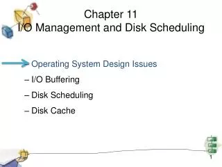
Overview • Review of I/O Techniques • I/O Buffering • Disk Geometry • Disk Scheduling Algorithms • RAID
Review • Input / Output techniques • Programmed I/O • Interrupt Driven I/O • Direct Memory access • I/O Layering • Application • Device Independent I/O • Driver • Interrupt Service Routine
I/O Buffering • Advantages • Overlap I/O and computation • Separates I/O from computation e.g. I/O can occur even if buffer is swapped • Time measurement parameters • T = I/O transfer time • C = computation time • M = block move time • Effect of buffering on program performance
No Buffers: T + C T Disk CPU User Copy C Disk CPU User Copy
One Buffer: max(T, C) + M C T CPU Disk System Buffer User Copy M CPU Disk System Buffer User Copy
Two Buffers: max(T, C + M) C CPU System Buffer 2 User Copy T Disk System Buffer 1 M CPU System Buffer 2 User Copy
I/O Buffering Summary • Buffering Alternatives • No buffering: T + C • Single buffer: max(T, C) + M • Double buffer: max(T, C + M) • Circular buffers: smooths out I/O demand • Disk cache - analogy to memory management • Fetch Policy - read ahead • Replacement choice: LRU, LFU, FIFO • When to do these: On demand or preplanned.
Classic Disk Geometry • Disk medium is a number of platters fixed to a axle spinning at high speed. • There is one read/write head for each surface of each platter. Heads are attached to an arm which varies by discrete amounts the distance to the axle of all heads simultaneously. • For each position of the arm, a head describes a circular track as the disk spins. Track is divided into segments called sectors which hold the data.
Disk Layout Intersector Gap Sector Track Intertrack Gap
Disk Performance • Seek time: time to move arm to right cylinder. Roughly linear in nbr. of tracks crossed: #tracks Trk2Trk + Startup. Average is seek over half the tracks. • Rotational delay: time to spin around to right sector on track • Access time: seek time + rotational delay • Transfer speed: how fast data spins past the head • Rotational speed and average seek time determine these parameters
Retail $100 IDE Disk Drive • Geometry • 8 platters (16 surfaces, 16 heads, 1 arm) • 7763 cylinders (7763 tracks per surface) • 63 sectors of 512 bytes each per track • Total: 16 7763 63 512 bytes = 3913 MB • Performance • Avg seek: 11 ms, Rotational speed: 5400 rpm • Avg rot. delay: 0.5/5400 min = 5.5 ms • Avg access time: 11 + 5.5 = 16.5 ms • trans speed: 63 5400 512 b/m = 2.8 MB/sec
Disk Scheduling Algorithms • FIFO - simple and fair • Priority • LIFO - serve current process well • Shortest service time first (SSTF) • SCAN - Back and forth over disk • C-SCAN - unidirectional scan • N-step SCAN - N jobs per queue • FSCAN - 2 queues
FIFO, Priority, and LIFO Disk Enter Disk Enter Enter Disk Enter
Shortest Service Time Next Jobs Entered In Sorted Order Disk 2 7 11 15 23 Numbers are Disk locations of data Select Closest Job 10 Current Location Starvation when arm is stuck in one area for extended period
Scan (Bidirectional) Jobs Entered In Sorted Order Disk 2 7 11 15 23 Scan Left to Right, Then Right to Left 10 Current Location Uneven response time at ends of disk
C-Scan (Unidirectional) Jobs Entered In Sorted Order Disk 2 7 11 15 23 Scan Left to Right, Then Return to left 10 Current Location Can Still Exhibit Starvation
N-step-Scan Jobs entered in sorted groups of N jobs Case where N = 1 is FIFO Groups Serviced In FIFO Order Disk 2 7 11 15 23
F-Scan Jobs Queued in Sorted Order Queue Group Disk 2 7 11 15 23 Dequeue Group Roles of two groups swapped when current group of jobs serviced.
Basic Disks • Master boot record (MBR) • Located on first sector of primary drive • Boot code • Partition Table (Up to 4 Entries) • Location and size of partition • File system type (e.g. FAT32, NTFS) • Extended Partition is a file system type • Recursively contains MBR and Partitions itself • Partitions • File System begins with boot sector
Dynamic Disks (1 of 2) • Logical Disk Manager (LDM) Database • Single database for all drives – includes multipartition volume descriptions • Replicated with one copy on each dynamic drive • 1 MB in size, located at end of drive • Master Boot Record (MBR) • Describes System and Boot partitions • If none, single partition from MBR to LDM • Boot and legacy software can’t read LDM
Dynamic Disks (2 of 2) • LDM Structure • Private Header • GUID for dynamic drive and disk group name • Replicated at end of LDM • Table of Contents • 128 byte database records • Entries all have name and id • Partitions: size, offset, disk id, parent component • Components: parent volume (2 for mirrors) • Volume: size, state, GUID, drive hint • Disk: GUID • Transactional Log
RAID • Redundant Array of Independent Disks • Six flavors • Level 0: Disk striping • Level 1: Disk mirroring • Level 2: Small strips, ECC e.g. Hamming • Level 3: Small strips with parity • Level 4: Large strips, fixed parity drive • Level 5: Large strips, round robin parity • Disk Spanning (not RAID)
Striping and Mirroring Stripes are fast; but not redundant 0 1 2 3 4 5 6 7 8 9 10 11 12 13 14 15 16 17 18 19 Mirroring Provides Data Redundancy at cost of doubling number of drives Has Fast Read Access 0 0 1 1 2 2 3 3
Raid Levels 2 and 3 Small Byte-sized Strips Redundancy 0 1 2 3 4 C C 5 6 7 8 9 C C 10 11 12 13 14 C C 15 16 17 18 19 C C Disk arms are in lock step; each access involves all disk drives. Fast access for large individual jobs - high overhead for many small I/O’s. Level 2 avoided because of added cost.
Raid Levels 4 and 5 Large Strips with Parity Strip Single drive for parity stays very busy 0 1 2 3 4 P 5 6 7 8 9 P 10 11 12 13 14 P 15 16 17 18 19 P P 0 1 2 3 4 Round robin parity 5 P 6 7 8 9 10 11 P 12 13 14 15 16 17 P 18 19
RAID Level 4 and 5 • Redundancy Principle • Bit values for parity drive are sum mod 2 of the corresponding bits on other drives • When a block is changed, the new parity can be computed in terms of the old value of the parity: • new parity = sum of old & new value and old parity bit modulo 2 • So one write requires: 2 reads and 2 writes • Reading requires just one read
RAID 5 Sector Calculation • Assume: • RAID 5 with k drives and sector sized strips • Sector/Drive numbers zero based • Effective capacity is k-1 times the size of a single drive • RAID logical sector N location: • R = N % (k * (k - 1)) • Drive = R%(k-1) + ((R%(k-1)>=R/(k-1)) ? 1 : 0) • Sector = N / (k - 1) • Parity Drive = R / (k – 1)