Download
1 / 16
240 likes | 492 Views
Representing Motion. Chapter 2. 2.1 Picturing Motion. What kinds of motion can you describe? How do you know that an object has moved? Be specific. Let’s start at the very beginning… Straight Line Motion. Motion Diagrams.

E N D
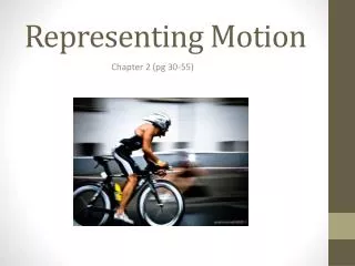
Representing Motion Chapter 2
2.1 Picturing Motion • What kinds of motion can you describe? • How do you know that an object has moved? Be specific. • Let’s start at the very beginning… Straight Line Motion.
Motion Diagrams • A series of images showing the positions of a moving object at equal time intervals is called a motion diagram. • A particle model is a simplified version of a motion diagram in which the object in motion is replaced by a series of single points.
2.2 Where and When? Beginning Vectors • Coordinate Systems • Tells you the location of the zero point of the variable you are studying and the direction in which the values of the variable increase. • The origin is the point at which both variables have a value of zero • Position can be represented by drawing an arrow from the origin to the point representing the object’s new location • The length of the arrow indicates how far the object is from the origin or the distance.
Vectors and Scalars Vectors Scalars • Have magnitude (size) and direction • Require the use of VECTOR ADDITION to determine resultant vector • Only have magnitude • Can be added or combined using standard rules of addition and subtraction
Vector Addition (Graphical Method) • You will need a ruler, protractor, and pencil • Draw a coordinate system (small) as your origin • Draw an arrow with the tail at the origin and the head pointing in the direction of motion. • The length of the arrow should represent the distance traveled. • Add the second vector using the head to tail method. • Measure resultant magnitude and direction.
Vector Addition (Geometry and Trig) • Add vectors using “head to tail” method. • Pictures do not need to be drawn to scale. No need for a ruler and protractor. • Use Pythagorean Theorem and SOHCAHTOA to solve for resultant vectors ONLY when RIGHT TRIANGLES are formed. • If not right triangles, use Law of Sines and Law of Cosines to solve for resultant vectors.
Time Intervals and Displacements • The difference between two times is called a time interval and is expressed as • i and f can be any two time variables you choose (according to each problem) • A change in position is referred to as displacement.
Displacement Ins and Outs • Distance ≠ Displacement • Displacement is the shortest distance from start to finishor “as the crow flies” • Draw the following: • 10m East • -10m • 10m North + 12m West
Vector Components • Every vector has x- and y- components. • In other words, a vector pointing southwest has both a south (y) and west (x) component. • Vectors can be “resolved into c0mponents”. • Use SOHCAHTOA to find the x- and y- components
Vector Addition (x- y- Component Method) • Break EACH vector into x- and y- components. • Assign negative and positive values to each component according to quadrant rules. For instance, south would have a negative sign. • Add the x- column. Add the y- column. • Use Pythagorean Theorem to determine the final displacement magnitude. • Use SOHCAHTOA to find the final displacement direction.
2.3 Position – Time Graphs • Plot time on the x-axis and position on the y-axis • Slope will indicate average velocity • Use this website for extra help. http://www.physicsclassroom.com/Class/1DKin/U1L3a.cfm
2.4 How Fast? • Average velocity is defined as the change in position, divided by the time during which the change occurred. • On a position vs. time graph, both magnitude and relative direction of displacement are given. A negative slope indicates an object moving toward the zero position. Speed simply indicates magnitude or “how fast.” Velocity indicates BOTH magnitude and direction. In other words velocity tells you “how fast” and “where.”
Instantaneous Velocity • When solving for average velocity, two points for position and time are chosen for comparison. Individual changes in speed could have taken place within those intervals. • Instantaneous velocity represents the speed and direction of an object at a particular instant. • On a position-time graph, instantaneous velocity can be found by determining the slope of a tangent line on the curve at an given instant.
Expressing Motion in Terms of An Equation • So far, we have looked at motion diagrams, particle models, and graphs as a means of representing motion. • Equations are also quite useful. • Based on the equation y=mx +b, one final equation will be derived in this chapter. d = final position v = average velocity t = time interval di = initial position (based on y-intercept if using a graph)
Final Thoughts • Read Chapter 1! You will reinforce all of these concepts, drill them into your head and see more examples than I have given here. • Visit www.physicsclassroom.com This website offers great explanations of physics concepts. • Watch this video. It is a little boring but very helpful. http://www.youtube.com/watch?v=4J-mUek-zGw