Download

1 / 23
250 likes | 715 Views
Chapter 3 Mobile Radio Propagation Large-Scale Path Loss. 3.1 Introduction to Radio Wave Propagation. Electromagnetic wave propagation reflection diffraction scattering Urban areas No direct line-of-sight high-rise buildings causes severe diffraction loss

E N D
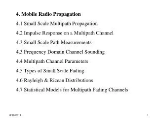
3.1 Introduction to Radio Wave Propagation • Electromagnetic wave propagation • reflection • diffraction • scattering • Urban areas • No direct line-of-sight • high-rise buildings causes severe diffraction loss • multipath fading due to different paths of varying lengths • Large-scale propagation models predict the mean signal strength for an arbitrary T-R separation distance. • Small-scale (fading) models characterize the rapid fluctuations of the received signal strength over very short travel distance or short time duration.
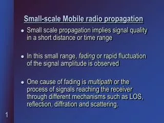
Small-scale fading: rapidly fluctuation • sum of many contributions from different directions with different phases • random phases cause the sum varying widely. (ex: Rayleigh fading distribution) • Local average received power is predicted by large-scale model (measurement track of 5 to 40 )
3.2 Free Space Propagation Model • The free space propagation model is used to predict received signal strength when the transmitter and receiver have a clear line-of-sight path between them. • satellite communication • microwave line-of-sight radio link • Friis free space equation : transmitted power : T-R separation distance (m) : received power : system loss : transmitter antenna gain : wave length in meters : receiver antenna gain
The gain of the antenna : effective aperture is related to the physical size of the antenna • The wave length is related to the carrier frequency by : carrier frequency in Hertz : carrier frequency in radians : speed of light (meters/s) • The losses are usually due to transmission line attenuation, filter losses, and antenna losses in the communication system. A value of L=1 indicates no loss in the system hardware.
Isotropic radiator is an ideal antenna which radiates power with unit gain. • Effective isotropic radiated power (EIRP) is defined as and represents the maximum radiated power available from transmitter in the direction of maximum antenna gain as compared to an isotropic radiator. • Path loss for the free space model with antenna gains • When antenna gains are excluded • The Friis free space model is only a valid predictor for for values of d which is in the far-field (Fraunhofer region) of the transmission antenna.
The far-field region of a transmitting antenna is defined as the region beyond the far-field distance where D is the largest physical linear dimension of the antenna. • To be in the far-filed region the following equations must be satisfied and • Furthermore the following equation does not hold for d=0. • Use close-in distance and a known received power at that point or
3.3 Relating Power to Electric Field • Consider a small linear radiator of length L
Electric and magnetic fields for a small linear radiator of length L with
At the region far away from the transmitter only and need to be considered. • In free space, the power flux density is given by • where is the intrinsic impedance of free space given by
The power received at distance is given by the power flux density times the effective aperture of the receiver antenna • If the receiver antenna is modeled as a matched resistive load to the receiver, the received power is given by
3.4 The Three Basic Propagation Mechanisms • Basic propagation mechanisms • reflection • diffraction • scattering • Reflection occurs when a propagating electromagnetic wave impinges upon an object which has very large dimensions when compared to the wavelength, e.g., buildings, walls. • Diffraction occurs when the radio path between the transmitter and receiver is obstructed by a surface that has sharp edges. • Scattering occurs when the medium through which the wave travels consists of objects with dimensions that are small compared to the wavelength.
Reflection from dielectrics • Reflection from perfect conductors • E-field in the plane of incidence • E-field normal to the plane of incidence
The actual received signal is often stronger than what is predicted by reflection and diffraction • Scattering • when a radio wave impinges on a rough surface, the reflected energy is spread out, e.g., trees, lamp posts. • Surface roughness is test using Rayleigh criterion which defines a critical height for a given angle of incidence
For rough surface, the flat surface reflection coefficient needs to be multiplied by a scattering loss factor is the standard deviation of the surface height.
3.5 Practical Link Budget Design using path Loss Models • Radio propagation models combine • analytical method • empirical method • Log-distance Path Loss Model • average received signal power decreases logarithmically with distance • The average path loss or
Log-normal Shadowing • Surrounding environmental clutter may be different at two different locations having the same T-R separation. • Measurements have shown that at any value d, the path loss PL(d) at a particular location is random and distributed normally (normal in dB) and : zero-mean Gaussian distributed random variable (in dB) with standard deviation • The probability that the received signal level will exceed a certain value can be calculated from where