Download
1 / 41
410 likes | 508 Views
Finding Motifs in Promoter Regions. Libi Hertzberg Or Zuk. Overview. Introduction and Definitions P-value Algorithm Experimental Results Generalizations and future work. REGULATOR. DNA. RNA polymerase. RNA polymerase. Transcription Factor (TF). Regulatory protein.

E N D
Finding Motifs in Promoter Regions Libi Hertzberg Or Zuk .
Overview • Introduction and Definitions • P-value Algorithm • Experimental Results • Generalizations and future work
REGULATOR DNA RNA polymerase RNA polymerase Transcription Factor (TF) Regulatory protein Regulatory protein Regulatory protein (singular) (complex) Regulatory protein TF binds Promoter motif Promoter motif mRNA of regulated gene Transcriptional Regulationin the cell:
Motif Representation We need to represent the motif – the TF binding site. There are three known representations: • Consensus – Most frequent letter in every position • IUPACcode – Allow all letters with frequency above a threshold in every position • Position Specific Weight Matrix – Count number of occurrences of every letter in every position - More Informative ! Known binding sites:
An Example: An alignment of 5 known binding sites of a TF Position Specific Weight Matrix - F
Giving a Score to a Potential Binding Site • We are given a site R=(r1,..., rL). We want to know how likely it is to be bound by the TF. We compute how well it fits to the weight matrix of the TF. • We do this by calculating the Likelihood function of the site – namely, the probability that it would have been generated given that it is indeed a binding site of this TF.
F = • Likelihood(“GATTCC”) = (3/5)*(1/5)*(5/5)*(2/5)*(4/5)*(1/5) = 0.00768
The Score • By taking log on the likelihood of R we get the score of R, which is the Loglikelihood of R. • Likelihood(“GATTCC”) = (3/5)*(1/5)*(5/5)*(2/5)*(4/5)*(1/5) = 0.00768 • score(“GATTCC”) = Loglikelihood(“GATTCC”) = log(3/5)+log(1/5)+log(5/5)+log(2/5)+log(4/5)+log(1/5) = -4.869
The PSSM • From the weight matrix F, we compute a Position Specific Score Matrix (PSSM) M by : • For example, MG,1 = log(3/5) F =
Finding The Motif We are given a TF and a gene. We want to know if this gene is regulated by the TF. Our Input : • The sequence of the promoter region of the gene • The PSSM of the TF A simple Algorithm : Scan the promoter region, and at each position calculate the score according to the PSSM. Take the best position (i.e. the one with the highest score) to be the suspected binding site. Max Score -2.3 -5.2 -4.5 -1.2 -0.5 AAGTTGCCGAGATCGTAGCTATCGATCGATCGACAGCTAAC
The Problem Problem : In any (e.g. random) sequence we will find some best position (and best score). How do we assign statistical significance(p-value) to the position and score we have found. Max Score -2.3 -5.2 -4.5 -1.2 -0.5 AAGTTGCCGAGATCGTAGCTATCGATCGATCGACAGCTAAC The Goal of Our Work Statistical Evaluation p value
Overview • Introduction and Definitions • P-value Algorithm • Experimental Results • Generalizations and future work
What Do We Want To Calculate? • Let N be the promoter length, and L the length of the TF binding site. Suppose we scanned the promoter and have found that the maximal score had the value t. • The p value is : the probability that the maximal score in a random sequence of length N, will be above the threshold t.
The Algorithm has two Steps : 1.Finding the set of all the sequences of lengthL, with a score above the thresholdt. 2. Calculate the probability of finding at least one of those sequences in a random sequence of length N.
Step One : Finding the sequences • Let K = K(t) be the number of sequences of length L (out of the 4L) with a score above t. • We have a branch and bound algorithm for enumerating them in time linear in K. • Problem : In some cases K might be too large. For example, Suppose L=20, and only one of a thousand sequences of length L has a score higher than t. It means K=420/1000 = 415 ~ 1billion.
Approximating K • If K is too large we cannot enumerate all the K sequences, but only try to estimate their number (i.e. K). • There are various methods to do so (Gaussian approximation, Statistical Mechanics, Large Deviations techniques). We used Generating Functions method, which proved to be the best. The method can give both lower and upper bounds on the correct number K.
Two Steps : 1. Finding the set of all the sequences of length L, with score above the threshold t. 2.Calculate the probability of finding at least one of those sequences in a random sequence of length N.
Step Two : Calculating Probabilities • We are given a set of K sequences. We need to calculate the probability of finding at least one of them in a random sequence of length N. • First, let’s consider a simpler problem, where we have one target R (K = 1).
Define : H – Number of occurrences of R in a promoter region of length N. R = • Our p value is : P(H > 0) = 1 – P(H = 0) AACG AAACGGTTGTTACAACGGTTCCTCCAACG H = 3
A Naive Approximation • At a specific position, the probability of R appearing is 1/4L, and the probability of R not appearing is (1 – 1/4L ) • A naive approximation : We have N-L+1 possible start positions, so : P(H = 0) ~ (1 – 1/4L )N-L+1 • Problem : We have neglected correlations !
Why Do Correlations Matter ? ATAA TAAA AAAA AAAC CTAA TAAC CAAA AAAG TAA AAA GTAA TAAG GAAA AAAT TTAA TAAT TAAA TAA appears in 8 sequences of length 4 P(H > 0) = 8/44 AAA appears in 7 sequences of length 4 P(H > 0) = 7/44 The Difference is in the self-overlapping pattern of them: TAATAAAAAAAA TAA TAAAAAAAA No Self overlaps :Maximal number of self overlaps: Less self overlaps Higher P(H>0)
The effect of self overlaps • The Mean of H Is : E(H) = (N-L+1) * (1/4L) Independent of the specific sequence R. • Proof:
TAAAAA AAAAAA The effect of self overlaps • The correlation between ‘close’ Xi’s depends on the specific sequence R. Less self overlaps Higher P(H>0) R1 = R2 =
Algorithm • We have developed a recursive algorithm which takes into account the correlations. It calculates the exact value of P(H > 0). • In the more interesting case, where we have a set of K target sequences, our method still applies. • If we assume that the promoter’s DNA is not random but there are different probabilities for A,T,C,G, the same algorithm still works. • Time Complexity : O(N * K log K)
Algorithm (Cont.) • When K is too large, we don’t know the exact sequences, but only (an approximation of) their number. • What we do : Take the worst-case scenario (i.e. highest P(H > 0) possible) • Highest p value : fewest overlaps. We assume no overlaps at all.
Algorithm (Cont.) • The case of no overlaps is possible for K < 4L/L. • We are usually interested in much smaller values of K. Thus, for our case of interest, the bound we get is quite tight. Upper Bound on P(H>0) -the P value! Upper Bound on K Lower Bound on Overlaps
Gene's Promoter Regions Sketch Of The System : Scan to get Max Scores Transcription Factors Weight Matrices Input Estimate K (For each pair!!) Small Large Enumerate K sequences FDR Bound pvalue Calculate pvalue p values Statistical Evaluation Statisticaly Significant Motifs Output
Overview • Introduction and Definitions • P-value Algorithm • Experimental Results • Generalizations and future work
A Comparison with Matinspector We used the Promoter Database of Saccharomyces cerevisiae. It contains genes and for every gene the TFs that are known to bind its promoter. We took 24 Transcription Factors whose PSWM is known, and 135 promoters of genes which are known to be bound by at least one of them. Our Results: We calculated the p-value (using the algorithm) for each of the TFs on each of the genes.
Our Results Each gene has 25 p-values of all the TFs. We used the FDR method to find the statistical significant TFs for every gene. Here the threshold for the FDR is 0.1, but we will check the results for a range of threshold values
Our Results • After we found statistical significant TFs for every gene, we compared the results with the data from the database. There are 2 parameters: • False positives rate – TFs that we found as statistical significant, but are not known to be bound to the gene. • False negatives rate – TFs that are known to be bound, but we didn’t find. Lower parameters values better results
Our Results Graph We calculated the average of these 2 parameters (False positives rate, false negatives rate) on all the genes, For a range of FDR threshold parameter values, Q = 0.01,…,0.45 Notice that the false positives rate is very close to the FDR threshold value
Matinspector Results • For every gene Matinspector gives the number of occurrences of every TF in its promoter, and an estimation of the expected number of occurrences (re value). • To compare to our results, we decided to declare a TF as significant if it was found more times than it is expected to be found, or, in other words, if the ratio (expected number)/(number of occurrences) is lower than a certain threshold.
Our Results Results Graphs Matinspector Results In our results the average of the 2 parameters (green) is always lower, And the false positives rate (red) is always much lower
Synthetic - 40% of positives are not annotated Real data Comparison with Synthetic Data Synthetic - All positives are annotated The left graph shows lower error rates then in our true data. The right graph shows error rates similar to those in our data, thus suggesting an estimate for the amount of missing real binding sites in the database.
Overview • Introduction and Definitions • P-value Algorithm • Experimental Results • Generalizations and future work
Markov Models • In true DNA sequences, the nucleotides are not independent but rather posses statistical dependencies at close distances. • To model this, we used a markov model, in which the distribution of each letter depends on some m previous ones. m is denoted as the size of the model. • Example : Each letter depends on it’s previous :
Markov Models (Cont.) • We can use this for both the binding site model and the background (‘random’) model. The more realistic the model, we hope to get more realistic p values. • We obtain a tradeoff. As we increase m : • Advantages : • More reliable p values • Reduce false positive/negative errors • Drawbacks : • Need more data to represent the model • Computational complexity increases
Other Possible Directions • Account for multiple occurrences: P(H = n). • Account for combinations of motifs. Find pairs (or larger groups) which are statistically significant. • Use close genomes (e.g. human and mouse) in order to reduce false positives rate. • Combine with expression data (how ?)
Ido Kanter Gaddy Getz Eytan Domany The END Thanks to