Download
1 / 62
620 likes | 788 Views
Latent Variable Methods in Process Systems Engineering. John F. MacGregor ProSensus , Inc. and McMaster University Hamilton, ON, Canada. www.prosensus.ca. OUTLINE. Presentation: Will be conceptual in nature Will cover many areas of Process Systems Engineering

E N D
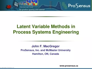
Latent Variable Methods in Process Systems Engineering John F. MacGregor ProSensus, Inc. and McMaster University Hamilton, ON, Canada www.prosensus.ca
OUTLINE • Presentation: • Will be conceptual in nature • Will cover many areas of Process Systems Engineering • Will be illustrated with numerous industrial examples • But will not cover any topic in much detail • Objective: • Provide a feel for Latent Variable (LV) models, why they are used, and their great potential in many important problems
Process Systems Engineering? • Process modeling, simulation, design, optimization, control. • But it also involves data analysis • learning from industrial data • An area of PSE that is poorly taught in many engineering programs • This presentation is focused on this latter topic • The nature of industrial data • Latent Variable models • How to extract information from these messy data bases for: • Passive applications: Gaining process understanding, process monitoring, soft sensors • Active applications: Optimization, Control, Product development • Will illustrate concepts with industrial applications
A. Types of Processes and Data Structures Batch Processes Data structures • Continuous Processes • Data structures End Properties time X1 variables X3 Y Z X Y batches X2 Initial Conditions Variable Trajectories
Nature of process data • High dimensional • Many variables measured at many times • Non-causal in nature • No cause and effect information among individual variables • Non-full rank • Process really varies in much lower dimensional space • Missing data • 10 – 30 % is common (with some columns/rows missing 90%) • Low signal to noise ratio • Little information in any one variable • Latent variable models are ideal for these problems
B. Concept of latent variables • Measurements are available on K physical variables: matrix=X • But, the process is actually driven by small set of “A” (A « K)independent latent variables,T. • Raw material variations • Equipment variations • Environmental (temp, humidity, etc.) variations Kcolumns = X
Projection of data onto a low dimensional latent variable space (T) Measured variables Latent variable space t2 t1 X T P Television analogy
X T Y P, W C Latent variable regression models X = TPT + E Y = TCT + F T = XW* Symmetric in X and Y • Both X and Y are functions of the latent variables, T • No hypothesized relationship between X and Y • Choice of X and Y is arbitrary (up to user) • A model exists for the X space as well as for Y (a key point)
Estimation of LV Model Parameters • Parameters: W*, C, P • Principal Component Analysis • Single matrix X: Maximizes the variance explained • PLS (Projection to Latent Structures / Partial Least Squares) • Maximizes covariance of (X, Y) • Reduced Rank Regression • Maximizes Var(Y) explained by X • Canonical Variate Analysis (CVA) • Maximizes correlation (X, Y) • Appear to be subtle differences, but method used is often critical to the application
Subspace IdentificationLatent variable methods you may be familiar with. • Subspace identification methods are latent variable methods • N4SID – Equivalent to Reduced Rank Regression (RRR) (maximizes the variance in Y explained thru correlation with X • CVA – Canonical Correlation Analysis (maximizes the correlation between X and Y) • State variables are the latent variables.
Important Concepts in Latent Variable Models • Handle reduced rank nature of the data • Work in new low dimensional orthogonal LV space (t1, t2,…) • Model for X space as well as Y space (PLS) • X = TPT + E ; Y = TCT + F • Unique among regression methods in this respect • X space model will be the key to all applications in this talk • Essential for uniqueness and for interpretation • Essential for checking validity of new data • Essential to handle missing data • Provide causal models in LV space • Optimization & control can be done in this space • only space where this is justified
Use of LV Models • Multivariate latent variable (LV) methods have been widely used in passive chemometric environments • A passive environment is one in which the model is only used to interpret data arising from a constant environment • Calibration • Inferential models (soft sensors) • Monitoring of processes • Used much less frequently in an active environment • An active environment is one in which the model will be used to actively adjust the process environment • Optimization • Control • Product Development
Causality in Latent Variable models • In the passive application of LV models no causality is required • Model use only requires that future data follow the same structure • No causality is implied or needed among the variables for use of the model • Calibration; soft sensors; process monitoring • For active use such as in optimization and control one needs causal models • For empirical models to be causal in certain x-variables – we need to have independent variation (DOE’s) in those x’s. • But much process modeling uses “happenstance data” that arise in the natural operation of the process • These models do not yield causal effects of individual x’s on the y’s • But LV models do provide causal models in the low dimensional LV space • ie. if we move in LV space (t1, t2, …) we can predict the causal effects of these moves on X and Y thru the X and Y space models • Will use this fact together with the model of the X-space to perform optimization and control in the LV spaces
C. Industrial applications • Analysis of historical data • Process monitoring • Inferential models / Soft sensors • Optimization of process operation • Control • Scale-up and transfer between plants • Rapid development of new products Passive applications Active applications
C. Industrial applications • Analysis of historical data • Process monitoring • Inferential models / Soft sensors • Optimization of process operation • Control • Scale-up and transfer between plants • Rapid development of new products Passive applications Active applications
Analysis of Historical Batch Data Batch Processes Data structure Herbicide Manufacture Z - Chemistry of materials - Discrete process events X - Process variable trajectories Y - Final quality - 71 batches ~ 400,000 data points End Properties time variables Z X Y batches Initial Conditions Variable Trajectories
Mean centering removes the average trajectories Models the time varying covariance structure among all the process variables over the entire time history of the batch Every batch summarized by a few LV scores (t1, t2, t3) Relates the IC’s (Z) and time varying trajectory information (X) to the final product quality (Y) Multi-way PLS for batch data
LV score plot for Z LV score plot for X Loading vector w*1 for X model VIP’s for Z model
C. Industrial applications • Analysis of historical data • Process monitoring • Inferential models / Soft sensors • Optimization of process operation • Control • Scale-up and transfer between plants • Rapid development of new products Passive applications Active applications
On-line Monitoring of New Batches • Multivariate Statistical Process Control • Build LV model on all acceptable operational data • Statistical tests to see if new batches remain within that model space • Hotelling’s T2 shows movement within the LV plane • SPE shows movement off the plane
Process monitoring: Herbicide process Monitoring of new batch number 73 T2 plot SPE plot
Contribution plots to diagnose the problem Problem: Variable x6 diverged above its nominal trajectory at time 277
C. Industrial applications • Analysis of historical data • Process monitoring • Inferential models / Soft sensors • Optimization of process operation • Control • Scale-up and transfer between plants • Rapid development of new products Passive applications Active applications
Image-based Soft Sensor for Monitoring and Feedback Control of Snack Food Quality Lab Analysis
PCA Score Plot Histograms Non-seasoned Low-seasoned High-seasoned
Segment Score Space into Multi-mask Region Based on Covariance with Quality Score space divided up into 32 regions corresponding to various coating levels
Distribution of Pixels Superposition of the score plots from 3 sample images on top of the mask Non-seasoned Low-seasoned High-seasoned Distribution of pixels Cumulative distribution of pixels
Model to Predict Seasoning Concentration Feature Extraction PLS Regression X Y Cumulative Histogram Color Images Seasoning Measurements Model for Seasoning Level
Seasoning level Non-seasoned Low-seasoned High-seasoned Visualize Images: Pixel by pixel Prediction of Seasoning Concentration
Online Results: Mixed Product Experiment Predicted seasoning level Predicted seasoning distribution variance
C. Industrial applications • Analysis of historical data • Process monitoring • Inferential models / Soft sensors • Optimization of process operation • Control • Scale-up and transfer between plants • Rapid development of new products Passive applications Active applications
Optimizing operating policies for new products Temperatures Pressures Concentrations Recipes Flows Trajectories X Y Density Tensile strength Mw, Mn Transparency Biological activity Toxicity Hydrophobicity
Batch polymerization: Process trajectory data (X) Batch polymerization – Air Products & Chemicals
Batch polymerization data • 13 variables in Y Desire a new product with the following final quality attributes (Y’s): • Solution • Build batch PLS latent variable model on existing data • Perform an optimization in LV space to find optimal LV’s • Use LV model of X-space to find the corresponding recipes and process trajectories • Maintain in normal ranges: Y1 Y2 Y3 Y4 Y5 Y6 Y8 • Constraints: Y7 = Y7des • Y9 = Y9des • Y10< Y10const • Y11< Y11const • Y12 < Y12const • Y13 < Y13const • … and with the minimal possible batch time (*)
PLS Model: Unconstrained Solution • Design via PLS model inversion (no constraints) • If dim(Y) < dim(X) then there is a null space • A whole line or plane of equivalent solutions yielding the same ydes Step 1 Step 2
Solution with constraints: Formulate inversion as an optimization • Step 1: Solve for with constraints on T2 and on y’s • Step 2: Solve for xnew that yields subject to certain constraints on SPE and x’s.
Different solutions: change the penalty () on time usage All solutions satisfy the requirements on ydes Case 1 to 5: weight on time-usage is gradually increased • Garcia-Munoz, S., J.F. MacGregor, D. Neogi, B.E. Latshaw and S. Mehta, “Optimization of batch operating policies. Part II: Incorporating process constraints and industrial applications”, Ind. & Eng. Chem. Res., 2008
C. Industrial applications • Analysis of historical data • Process monitoring • Inferential models / Soft sensors • Optimization of process operation • Control • Scale-up and transfer between plants • Rapid development of new products Passive applications Active applications
Control of batch product quality • Objective is to control final product quality • e.g. control of final particle size distribution (PSD) • Using all data up to some decision time, predict final quality with latent variable model • All prediction done in low dimensional latent variable space (y’s then calculated from t’s) • If predicted quality is outside a desired window, then make a mid-course correction to the batch • Analogy to NASA mid-course rocket trajectory adjustment in moon missions • Data requirement: Historical batches + few with DOE on corrective variables
LV models provide accurate adaptive trajectory predictions • Use various missing data imputation methods • - Equivalent of Kalman Filter Prediction of a variable trajectory using information up to time 30 (DuPont) Deviations from the mean trajectory – Prediction vs actual
Heat release trajectories from different batches Decision point Action Time interval Control of PSD via mid-course correction • At decision point – predict t’s (Y’s) – if outside target region – take action Predicted final t’s ? t2 t1
Industrial results (Mitsubishi Chemicals) Mid-course control : before and after implementation
C. Industrial applications • Analysis of historical data • Process monitoring • Inferential models / Soft sensors • Optimization of process operation • Control • Scale-up and transfer between plants • Rapid development of new products Passive applications Active applications
Product transfer between plants and scale-up Target site Source site Process conditions Process conditions Chemical or physical properties for each product Chemical or physical properties for each product Product 4 Product 1 Product 5 Product 2 Product 3
Xa Ya Xb Yb Product transfer and scale-up Historical data from the 2 plants. Build JYPLS model T T ybdesT xbnewT Y space model X space model Garcia-Munoz, S., T.Kourti and J.F. MacGregor, “Product Transfer Between Sites using Joint-Y PLS”, Chemometrics & Intell. Lab. Systems, 79, 101-114, 2005.
Industrial Scale-up Example Tembec - Cdn. pulp & paper company: Pilot plant and full scale digesters
Scale up for grade F – pulp digester • Build models on all pilot plant data and all plant data (ex F) • Design operating profiles to achieve grade F in plant. Predicted trajectory Actual plant trajectory used to achieve the grade
C. Industrial applications • Analysis of historical data • Process monitoring • Inferential models / Soft sensors • Optimization of process operation • Control • Scale-up and transfer between plants • Rapid development of new products Passive applications Active applications