Download

1 / 65
670 likes | 974 Views
MS Excel 2003. Part 1 Ms Saima Gul. What is Excel?. Excel 2003 is the spreadsheet and data analysis program in Office 2003. It combines incredible power with ease of use, giving professionals and occasional users the features they need. What is Excel Used For?.

E N D
MS Excel 2003 Part 1 Ms Saima Gul
What is Excel? • Excel 2003 is the spreadsheet and data analysis program in Office 2003. It combines incredible power with ease of use, giving professionals and occasional users the features they need.
What is Excel Used For? • Number crunching: Create budgets, analyze survey results, and perform just about any type of financial analysis you can think of. • Creating charts: Create a wide variety of highly customizable charts. • Organizing lists: Use the row-and-column layout to store lists efficiently. • Accessing other data: Import data from a wide variety of sources. • Creating graphics and diagrams: Use Excel AutoShapes to create simple (and not-so-simple) diagrams.
Excel Elements • Windows elements • Menus, shortcut keys, toolbars, dialogs and task panel • Document scrolling techniques • Help feature
Menu bar Excel Environment Formula bar Column heading Cell pointer Row heading sheet tabs
Understanding Workbooks and Worksheets • The work you do in Excel is performed in a workbook file, which appears in its own window. You can have as many workbooks open as you need. By default, workbooks use an XLS file extension. • Each workbook is comprised of one or more worksheets, and each worksheet is made up of individual cells. Each cell contains a value, a formula, or text. Each worksheet is accessible by clicking the tab at the bottom of the workbook. In addition, workbooks can store chart sheets. A chart sheet displays a single chart and is also accessible by clicking a tab.
Working with Workbooks • Excel 2003 automatically starts with a new Workbook containing three Worksheets. • A Workbook consists of one or more Worksheets. • A Worksheet is essentially a very large table, consisting of rows and columns.
Moving Around a Worksheet • Every worksheet consists of rows (numbered 1 through 65,536) and columns (labeled A through IV). After column Z comes column AA; after column AZ comes column BA, and so on. The intersection of a row and a column is a single cell. At any given time, one cell is the active cell. You can identify the active cell by its darker border. Its address (its column letter and row number) appears in the Name box. Depending on the technique that you use to navigate through a workbook, you may or may not change the active cell when you navigate.
Working with Cells • A Worksheet is made up of Cells. A Range is made up of Cells. Ranges can be any rectangular area of Cells within a Worksheet. • Excel identifies the Active Cell with a bold outline around the Cell and highlighting the Column heading letter and Row heading number of the Cell.
Navigating within a Worksheet • A common way to navigate within a Worksheet is to use your keyboard.
Selecting Items in Excel • Select a Column by clicking on the Column header letter. • Select a Row by clicking on the Row header number. • Select a Range by clicking on the First Cell; hold down the Shift key and click the Opposing Cell in the Range.
Modifying Cell Contents • After you enter a value or text into a cell, you can modify it in several ways: • Erase the cell’s contents • Replace the cell’s contents with something else • Edit the cell’s contents
Erasing the contents of a cell • To erase the contents of a cell, just click the cell and press Delete. To erase more than one cell, select all the cells that you want to erase and then press Delete. Pressing Delete removes the cell’s contents but doesn’t remove any formatting (such as bold, italic, or a different number format) that you may have applied to the cell. • For more control over what gets deleted, you can use the Edit➪Clear command. This menu item has a submenu with four additional choices: • All: Clears everything from the cell • Formats: Clears only the formatting and leaves the value, text, or formula • Contents: Clears only the cell’s contents and leaves the formatting • Comments: Clears the comment (if one exists) attached to the cell
Editing the contents of a cell • When you want to edit the contents of a cell, you can use one of the following ways to enter cell-edit mode: • Double-click the cell. This enables you to edit the cell contents directly in the cell. • Activate the cell and press F2. This enables you to edit the cell contents directly in the cell. • Activate the cell that you want to edit and then click inside the Formula bar. This enables you to edit the cell contents in the Formula bar. • All of these methods cause Excel to go into edit mode. (The word EDIT appears at the left side of the status bar at the bottom of the screen.) When Excel is in edit mode, the Formula bar displays two new icons: the X and Check Mark. Clicking the X icon cancels editing, without changing the cell’s contents. (Pressing Esc has the same effect.) Clicking the Check Mark icon completes the editing and enters the modified contents into the cell. (Pressing Enter has the same effect.)
To name a worksheet • In the lower left corner of the workbook window, right-click the desired sheet tab. • From the shortcut menu that appears, click Rename. • Type the new name for the worksheet, and press Enter. To reposition a worksheet • Click the sheet tab of the worksheet you want to move, and drag it to the new position on the tab bar.
To change the default number of worksheets • On the Tools menu, click Options. • In the Options dialog box, click the General tab, and, in the Sheets In New Workbook box, type the number of worksheets you want in your new workbooks. • Click OK.
To merge cells • Select the cells to be merged. • On the Formatting toolbar, click the Merge and Center toolbar button. To add cells to a worksheet • On the Insert menu, click Cells. • In the Insert dialog box, select the option button indicating whether to shift the cells surrounding the inserted cell down (if your data is arranged as a column) or to the right (if your data is arranged as a row). • Click OK.
To delete cells from a worksheet • Select the cells to delete and, on the Edit menu, click Delete. • In the Delete dialog box, select the option button indicating whether to shift the cells surrounding the deleted cells up (if your data is arranged as a column) or to the left (if your data is arranged as a row). • Click OK.
Inserting rows and columns • To insert a new row or rows, you can use any of the following techniques: • Select an entire row or multiple rows by clicking the row numbers in the worksheet border. Select the Insert➪Rows command. • Select an entire row or multiple rows by clicking the row numbers in the worksheet border. Right-click and choose Insert from the shortcut menu. • Move the cell pointer to the row that you want to insert and then select Insert➪Rows. If you select multiple cells in the column, Excel inserts additional rows that correspond to the number of cells selected in the column and moves the rows below the insertion down. • The procedure for inserting a new column or columns is similar, but you use the Insert➪Column command.
Deleting rows and columns • To delete a row or rows, use any of the following methods: • Select an entire row or multiple rows by clicking the row numbers in the worksheet border and then select Edit➪Delete. • Select an entire row or multiple rows by clicking the row numbers in the worksheet border. Right-click and choose Delete from the shortcut menu. • Move the cell pointer to the row that you want to delete and then select Edit➪Delete. In the dialog box that appears, choose the Entire row option. If you select multiple cells in the column, Excel deletes all selected rows. • Deleting columns works in a similar way.
Hiding rows and columns • If necessary, you can hide rows and columns. This may be useful if you don’t want users to see particular information or if you need to print a report that summarizes the information in the worksheet without showing all the details. • To hide rows or columns in your worksheet, select the row or rows that you want to hide and then choose Format➪Row➪Hide. Or select the column or columns that you want to hide and then choose Format➪Column➪Hide. • Unhiding a hidden row or column can be a bit tricky because selecting a row or column that’s hidden is difficult. The solution is to select the columns or rows that are adjacent to the hidden column or row. (Select at least one column or row on either side.) Then select Format➪Row➪Unhide or Format➪Column➪Unhide. Another method is to select Edit➪Go To (or its F5 equivalent) to select a cell in a hidden row or column. For example, if column A is hidden, you can press F5 and specify cell A1 (or any other cell in column A) to move the cell pointer to the hidden column. Then you can use the appropriate command to unhide the column.
Changing column widths • You can change columns widths by using anyof the following techniques. • Drag the right-column border with the mouse until the column is the desired width. • Choose Format➪Column➪Width and enter a value in the Column Width dialog box. • Choose Format➪Column➪AutoFit Selection. This adjusts the width of the selected column so that the widest entry in the column fits. If you want, you can just select cells in the column, and the column is adjusted based on the widest entry in your selection. • Double-click the right border of a column header to set the column width automatically to the widest entry in the column.
Changing row heights • Drag the lower row border with the mouse until the row is the desired height. • Choose Format➪Row➪Height and enter a value (in points) in the Row Height dialog box. • Double-click the bottom border of a row to set the row height automatically to the tallest entry in the row. You also can use the Format➪Row➪AutoFit command for this.
To prevent text spillover • Click the desired cell. • On the Format menu, click Cells. • If necessary, click the Alignment tab. • Select the Wrap Text check box, and click OK.
Formatting numbers by using the toolbar • The Formatting toolbar contains several buttons that let you quickly apply common number formats. When you click one of these buttons, the active cell takes on the specified number format. You also can select a range of cells (or even an entire row or column) before clicking these buttons. If you select more than one cell, Excel applies the number format to all the selected cells. Table on next slide summarizes the formats that these Formatting toolbar buttons perform.
To add a picture to a worksheet • Click the cell into which you want to add the picture. • On the Insert menu, point to Picture and then click From File. • Navigate to the folder with the picture file, and then double-click the file name. To change a picture’s properties • Right click the graphic and from the shortcut menu that appears, click Format Picture. • Use the controls in the Format Picture dialog box to change the picture’s properties.
To add a background image to a worksheet • On the Format menu, point to Sheet, and click Background. • In the Sheet Background dialog box, click the image that you want to serve as the background pattern for your worksheet, and click OK.
Formatting Text • You can format your text using the Font tab of the Format Cell dialog box.
Formatting Numbers • You can format your numbers using the Number tab of the Format Cell dialog box. • Or use the icons on the Formatting toolbar.
Manipulating Data • The Alignment tab of the Format Cells dialog gives you great control over how your text is aligned and orientated.
Formatting with Colours and Patterns • You can customize your spreadsheets by changing the Font Colour or by adding a Fill Colour or Pattern. (Right click -> Format Cells -> Patterns)
Adding and Editing Borders • The Border tab of the Format Cell dialog box provides many options to customise your borders.
Using AutoFormat • Excel 2003 has many pre-defined table styles to help you format your table of information quickly. (Format -> Auto Format)
Using Page Setup • You can use the Page Setup dialog to customize the printing of your Spreadsheet. (File -> Page Setup)
Margins • Use the Margin tab of the Page Setup dialog box to define margins and centre data on the printed page.
Headers and Footers • Use the Header/Footer tab to add standard or custom Header and Footer.
Understanding the Types of Data You Can Use • An Excel workbook can hold any number of worksheets, and each worksheet is made up of a large number of cells. A cell can hold any of three basic types of data: • Numerical values • Text • Formulas • A worksheet also can hold charts, drawings, pictures, buttons, and other objects. These objects are not contained in cells. Rather, they reside on the worksheet’s draw layer, which is an invisible layer on top of each worksheet.
Understanding numerical values • Numerical values represent a quantity of some type: sales amounts, number of employees, atomic weights, test scores, and so on. Values also can be dates (such as 26-Feb-2004) or times (such as 3:24 a.m.).
Understanding text entries • Most worksheets also include text in some of their cells. You can insert text to serve as labels for values, headings for columns, or instructions about the worksheet. Text is often used to clarify what the values in a worksheet mean. In most cases, the text is more important to someone viewing the worksheet than it is to Excel because the text makes it easier for the viewer to determine which numerical values are which—Excel knows what the values represent from the way that they are used in formulas. • Text that begins with a number is still considered text. For example, if you type 12 Apples into a cell, Excel considers this to be text rather than a value. Consequently, you can’t use this cell for numeric calculations.
Understanding formulas • Formulas are what make a spreadsheet a spreadsheet. Excel enables you to enter powerful formulas that use the values (or even text) in cells to calculate a result. When you enter a formula into a cell, the formula’s result appears in the cell. If you change any of the values used by a formula, the formula recalculates and shows the new result. • Formulas can be simple mathematical expressions, or they can use some of the powerful functions that are built into Excel.
Forcing text to appear on a new line within a cell • If you have lengthy text in a cell, you can force Excel to display it in multiple lines within the cell. Use Alt+Enter to start a new line in a cell.
Entering numbers with fractions • To enter a fraction into a cell, leave a space between the whole number and the fraction. For example, to enter 6 ¾, enter 6 3/4, and then press Enter. When you select the cell, 6.75 appears in the Formula bar, and the cell entry appears as a fraction. • If you have a fraction only (for example, ¼), you must enter a zero first, like this: 0 1/4—otherwise Excel will likely assume that you are entering a date. When you select the cell and look at the Formula bar, you see 0.25. In the cell, you see ¼.
Hiding and unhiding a worksheet • In some situations, you may want to hide one or more worksheets. Hiding a sheet may be useful if you don’t want others to see it, or if you just want to get it out of the way. When a sheet is hidden, its sheet tab is also hidden. At least one sheet must remain visible. (You can’t hide all the sheets in a workbook.) • To hide a worksheet, choose Format➪Sheet➪Hide. The active worksheet (or selected worksheets) will be hidden from view.
Keeping the titles in view by freezing panes • If you set up a worksheet with row or column headings, it’s easy to lose track of just where you are when you scroll to a different location in the worksheet. Excel provides a handy solution to this problem: freezing panes. This keeps the headings visible while you are scrolling through the worksheet. • To freeze panes, start by moving the cell pointer to the cell below the row that you want to remain visible as you scroll and to the right of the column that you want to remain visible as you scroll. Then, select Window➪Freeze Panes. Excel inserts dark lines to indicate the frozen rows and columns. You’ll find that the frozen row and column remain visible as you scroll throughout the worksheet. To remove the frozen panes, select Window➪Unfreeze Panes.
Monitoring cells with a Watch Window • In some situations, you may want to keep track of the value in a particular cell. As you scroll throughout the worksheet, that cell may disappear from view. Using a Watch Window can help. • The Watch Window is actually a special type of toolbar. To display the Watch Window toolbar, choose View➪Toolbars➪Watch Window. Then click Add Watch and specify the cell that you want to watch. The Watch Window will display the value in that cell. You can add any number of cells to the Watch Window, and you can move the toolbar to a convenient location.
Pasting in special ways • To control what is copied into the destination range, you use the Edit➪Paste Special command—a much more versatile version of the Edit➪Paste command. This dialog box has several options, which are explained in the following list. • All: Equivalent to using the Edit➪Paste command. It copies the cell’s contents, formats, and data validation from the Windows Clipboard. • Formulas: Only formulas contained in the source range are copied. • Values: Copies the results of formulas. • Formats: Copies only the formatting. • Comments: Copies only the cell comments from a cell or range. This option doesn’t copy cell contents or formatting.