Download
1 / 19

E N D
1. Caustics Generation by using Photon Mapping Presentation by Michael Kaiser and Christian Finger
Advised by Dr. Marcus Magnor
13.02.2004
Light and Color in Nature Seminar,
Max-Planck-Institut f�r Informatik
2. Motivation Create nice pictures with translucent objects and rendering nice effects on diffuse surfaces.
3. Overview Caustics
Photon Mapping
Results
4. Light Transport Notation L Lightsource
E Eye
S Specular reflection
D Diffuse reflection
(k)+ one or more k events
(k)* zero or more of k events
(k)? zero or one k event
(k|k�) a k or k� event
5. Caustics Caustics are formed when light reflected from or transmitted through one or more specular surfaces strikes a diffuse surface.
In Light transport notation: LS+DE
6. Comparisons Classical Ray Tracing
LD?S*E
Does not support Caustics.
Path Tracing
L(S|D)*E
Would be qualified for simulating caustics.
But: Probability of going through a series of LS+DE is small.
Bidirectional Path Tracing
L(S|D)*E
Would be also qualified for simulating caustics.
Produces correct pictures, unbiased solution.
Takes too much time for same quality as photon mapping.
7. Comparisons Radiosity
Handles only diffuse reflections LD*E.
Not suitable for rendering caustics.
Photon Mapping
Handles all kinds of reflections.
It has the following possibilities: L(S|D)*D
Good for Caustics.
8. 2-Pass Algorithm First Pass:
Generating a Global Photon Map and Caustic Map.
9. Photon Maps Global Photon Map
All Photons with property L(S|D)*D are stored.
Caustic Map
Only Photons with paths LS+D are directly stored.
Application of a projection map.
10. Photon Mapping Rendering equation is solved by a photon map.
Density estimation
11. Photon Mapping For the rendering part incoming radiance is divided into four parts:
12. Photon Mapping
13. Photon Mapping
14. Results
15. Results
16. Results
17. Outlook Rendering participating media
Additional Volume Photon Map.
Rendering Volume Caustics.
18. Literature Henrik Wann Jensen, �Realistic Image Synthesis Using Photon Mapping�, A.K. Peters, 2001
19. Questions?