Download
1 / 28
280 likes | 422 Views
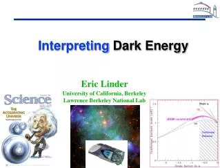
Course on Dark Energy Cosmology at the Beach 2009. Eric Linder University of California, Berkeley Lawrence Berkeley National Lab. JDEM constraints. Outline. Lecture 1: Dark Energy in Space The panoply of observations Lecture 2: Dark Energy in Theory The garden of models

E N D
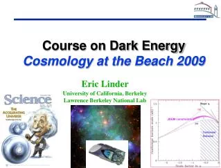
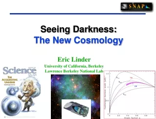
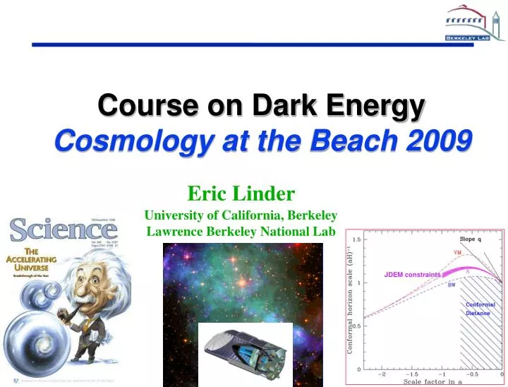
Course on Dark Energy Cosmology at the Beach 2009 Eric Linder University of California, Berkeley Lawrence Berkeley National Lab JDEM constraints
Outline Lecture 1: Dark Energy in Space The panoply of observations Lecture 2: Dark Energy in Theory The garden of models Lecture 3: Dark Energy in your Computer The array of tools– Don’t try this at home! In theory, there is no difference between theory and practice. In practice, there is. - Yogi Berra
Solving the Equation of Motion Klein-Gordon equation Transform to new variables Autonomous system Copeland, Liddle, Wands 1998 Phys. Rev. D 57, 4686 where Transform solution to Can add equation for EOS dynamics Caldwell & Linder 2005 Phys. Rev. Lett 95, 141301
Equation of State Dynamics For robust solutions, pay attention to initial conditions, shoot forward in time, use 4th order Runge-Kutta. For monotonic , can switch to as time variable, defining present as, e.g. =0.72.
Asymptotic Behaviors Asymptotic behaviors can be physically interesting. Solve for critical pointsx(xc,yc)=0, y(xc,yc)=0. Check stability by sign of eigenvalues p=Mp. p={x,y} Copeland, Liddle, Wands 1998 Phys. Rev. D 57, 4686 Relevant to fate of universe. Crossing w=-1: Phantom fields roll up potential so V>0, so wtot∞<-1. Cannot cross w=-1 even with coupling. Quintessence can cross with coupling since w<wtot.
From Data to Theory (and back) ( ) ) ( 2() COV(,w) COV(,w)2(w) F Fw Fw Fww C = F-1 = F = Fisher matrix gives lower limit for Gaussian likelihoods, quick and easy. Fij = d2(- ln L) / dpi dpj = O(dO/dpi) COV-1 (dO/dpj) (pi) 1/(Fii)1/2 Example: O=dlum(z=0.1,0.2,…1), p=(m,w), COV=(d/d)d ij Fw=k(dOk/d)(dOk/dw)k-2 See: Tegmark et al. astro-ph/9805117 Dodelson, “Modern Cosmology” Also called information matrix. Add independent data sets, or priors, by adding matrices. e.g. Gaussian prior on m=0.280.03 via2 = (m-0.28)2/0.032
Survival of the Fittest Fisher estimates give a N-dimension ellipsoid. Marginalize (integrate over the probability distribution) over parameters not of immediate interest by crossing out their row/column in F-1.Fixa parameter by crossing out row/column in F. 1 (68.3% probability enclosed) joint contours have 2=2.30 in 2-D (not 2=1). Read off 1 errors by projecting to axis and dividing by 1.52=2.30. Orientation/ellipticity of ellipse shows degree of covariance (degeneracy). Different types of observations can have different degeneracies (complementarity) and combine to give tight constraints.
Bias from Systematics Fisher estimation calculated around fiducial model, but can also compute bias due to offset (systematic). Bias p in parameter p is related to offset O in observable, through U=O/p and covariance matrix C=O O. For diagonal covariance, simplifies to: In statistics, often combine uncertainty and bias into Risk parameter: R(p) = [2(p)+p2]1/2
Design an Experiment . Precision in measurement is not enough - one must beware degeneracies and systematics. Degeneracy: e.g. Aw0+Bwa=const Degeneracy: hypersurface, e.g. covariance with m p2 * or Systematic: floor to precision, e.g. calibration Systematic: offset error in data or model, e.g. evolution p1
Orthogonal Basis Analysis Eigenmodes: w(z) = i ei(z) For orthogonal basis, errors (i) are uncorrelated. “Principal components”. Start with parameters {wi} in z bins. Diagonalize Fisher matrix F=ETDE: D is diagonal, rows of E give eigenvectors.NOTE:basis differs withmodel, experiment, and probe -- cannot directly compare. Huterer & Starkman 2003
Decorrelated Bins Bandpowers or decorrelated redshift bins diagonalize sqrt{F} to try to localize w(zi). Unlike for LSS, for dark energy they do not localize well, and confuse interpretation. Also depends strongly on assumption of w(z>zmax)
Principal Component Analysis The uncertainties (i) have no physical meaning -- must interpret the signal-to-noise, not just the noise. Even next generation experiments have only 2 components with S/N>3. Almost all models have 97-100% of the information in first 2 components. Eigenmode analysis does not improve over w0-wa.
Common Mistakes • Neglecting M or S (SN or BAO absolute scale). • Neglecting systematics. • Claiming systematics, but still ’ing down errors. • Thinking “self calibration” covers systematics; “self calibration” = “assuming a known form”. • Using noise, not S/N, for PCA. • Fixing w=-1 at high redshift. • Reductio ad absurdum: • 1 SN/sec, 10 y survey gives d(z) to 0.003% • Every acoustic mode gives d(z) to 0.1% • Full sky space WL takes 1% shears to 310-6 level
Controlling Systematics Controlling systematics is the name of the game. Finding more objects is not. Forthcoming experiments may deliver 100,000s of objects. But uncertainties do not reduce by 1/N. Must choose cleanest probe/data, mature method, with multiple crosschecks.
Battle Royale Astronomer Royal (Airy): “I should not have believed it if I had not seen it!” Astronomer Royal (Hamilton): “How different we are! My eyes have too often deceived me. I believe it because I have proved it.”
What makes SN measurement special?Control of systematic uncertainties Each supernova is “sending” us a rich stream of information about itself. Images Nature of Dark Energy Redshift & SN Properties Spectra data analysis physics
Astrophysical Uncertainties For accurate and precision cosmology, need to identify and control systematic uncertainties.
Controlling Systematics Same SN, Different z Cosmology Same z, Different SN Systematics Control
Fitting Subsets perfect
Depth + Width + Resolution Bacon, Ellis, Refregier 2000 Weak lensing noise Weak lensing signal Kasliwal, Massey, Ellis, Miyazaki, Rhodes 2007 Subaru - best ground HST - space
Cluster Abundances Clusters-- largest bound objects. DE + astrophysics.Uncertainty in mass of 0.1 dex gives wconst~0.1[M. White],w~? Xray: hot gas gravitational potential mass Optical: light mass Clean detections Difficult for z>1 Need optical survey for redshift Detects flux, not mass Only cluster center Assumes simple: ~ne2 Traditional Difficult for z>1 Detects light, not mass Mass of what? Sunyaev-Zel’dovich: hot e- scatter CMB mass Weak Lensing: gravity distorts images of background galaxies Clean detections Indepedent of redshift Need optical survey for redshift Detects flux, not mass Assumes ~simple: ~neTe Detect mass directly Can go to z>1 Line of sight contamination Efficiency reduced
Heterogeneous Data Offsets due to different instruments, filters, sources can be a serious source of bias. “Stitching together” surveys, even with modest overlap, may give precision cosmology, but inaccurate results. No need to stitch in z>2 – no leverage.
Design an Experiment • How to design an experiment to explore dark energy? • Choose clear, robust, mature techniques • Rotate the contours thru choice of redshift span • Narrow the contours thru systematics control • Break degeneracies thru multiple probes • Use homogeneous data set With a strong experiment, we can even test the framework of physics. Recall {m,w0,wa,,g*}.
Discovery Space • Dark energy may be a decades long mystery. • Space wide-field surveysmaximize the discovery space. • Fundamental physics of inflation: • Weak lensing - ns primordial perturbation spectrum • Cluster abundances - non-Gaussianity • Dark Matter maps - 40 trillion pixels on sky! 20x ground. “the skeleton of the universe” Imagine COSMOS x 2000!
Dark Energy – The Next Generation Euclid (ESA) Launch ~2015 104 the Hubble Deep Field area (and deeper) plus 107 HDF (almost as deep) w i d e deep Mapping 10 billion years / 70% age of universe colorful Optical + IR to see thru dust, to high redshift
The Next Physics Current data do not tell us is the answer (or anything about dark energy at z>1). Odds against: Einstein+us failed for 90 years to explain it. Experiments to reveal dynamics (w-w) are essential to reveal physics. Space is the low risk option for dependable answers. Expansion plus growth(e.g. SN+WL) is critical combination. We can test GR and can test geometry. Space imaging missiongives optical-NIR and low-high z measurements, high resolution and low systematics; multiple probes and rich astronomical resources. What is dark energy? What is the fate of the universe? How many dimensions are there? How are quantum physics and gravity unified?
Dark Energy Pessimism [2008 STScI Symposium: “We shall never be able to know the composition of dark energy” -- pessimistic physicist] 1835: “We shall never be able to know the composition of stars” -- Comte 1849: Kirchhoff discovers that the spectrum of electromagnetic radiation encodes the composition [2022? Cosmology on the Beach: Fiji has talks revealing the true nature of dark energy
“Acceleration” to the tune of The Beatles’ “Revolution”