Download
1 / 45
460 likes | 537 Views
Whole Genome Assembly Microarray analysis. Mate-pairs allow you to merge islands (contigs) into super-contigs. Mate Pairs. Make clones of truly predictable length. EX: 3 sets can be used: 2Kb, 10Kb and 50Kb. The variance in these lengths should be small.

E N D
Mate-pairs allow you to merge islands (contigs) into super-contigs Mate Pairs
Make clones of truly predictable length. EX: 3 sets can be used: 2Kb, 10Kb and 50Kb. The variance in these lengths should be small. Use the mate-pairs to order and orient the contigs, and make super-contigs. Super-contigs are quite large
40-50% of the human genome is made up of repetitive elements. Repeats can cause great problems in the assembly! Chimerism causes a clone to be from two different parts of the genome. Can again give a completely wrong assembly Repeats & Chimerisms
Repeat detection • Lander Waterman strikes again! • The expected number of clones in a Repeat containing island is MUCH larger than in a non-repeat containing island (contig). • Thus, every contig can be marked as Unique, or non-unique. In the first step, throw away the non-unique islands. Repeat
Detecting Repeat Contigs 1: Read Density • Compute the log-odds ratio of two hypotheses: • H1: The contig is from a unique region of the genome. • The contig is from a region that is repeated at least twice
Detecting Chimeric reads • Chimeric reads: Reads that contain sequence from two genomic locations. • Good overlaps: G(a,b) if a,b overlap with a high score • Transitive overlap: T(a,c) if G(a,b), and G(b,c) • Find a point x across which only transitive overlaps occur. X is a point of chimerism
Contig assembly • Reads are merged into contigs upto repeat boundaries. • (a,b) & (a,c) overlap, (b,c) should overlap as well. Also, • shift(a,c)=shift(a,b)+shift(b,c) • Most of the contigs are unique pieces of the genome, and end at some Repeat boundary. • Some contigs might be entirely within repeats. These must be detected
Supercontig assembly • Supercontigs are built incrementally • Initially, each contig is a supercontig. • In each round, a pair of super-contigs is merged until no more can be performed. • Create a Priority Queue with a score for every pair of ‘mergeable supercontigs’. • Score has two terms: • A reward for multiple mate-pair links • A penalty for distance between the links.
Supercontig merging • Remove the top scoring pair (S1,S2) from the priority queue. • Merge (S1,S2) to form contig T. • Remove all pairs in Q containing S1 or S2 • Find all supercontigs W that share mate-pair links with T and insert (T,W) into the priority queue. • Detect Repeated Supercontigs and remove
Repeat Supercontigs • If the distance between two super-contigs is not correct, they are marked as Repeated • If transitivity is not maintained, then there is a Repeat
Consenus Derivation & Assembly • Summary • Do an “all pairs” prefix-suffix alignment. (Speedup using k-mer hashing). • Construct a graph of overlapping alignments. • Break the graph into “unique” regions (Number of clones similar to prediction using LW), and “repeat/chimeric” regions. Each such “unique’ region is called a contig. • Merge contigs into super-contigs using mate-pair links • For each contig, construct a multiple alignment, and consensus sequence. • Pad the consensus sequence using NNs.
Summary • Once controversial, whole genome shotgun is now routine: • Human, Mouse, Rat, Dog, Chimpanzee.. • Many Prokaryotes (One can be sequenced in a day) • Plant genomes: Arabidopsis, Rice • Model organisms: Worm, Fly, Yeast • WGS must be followed up with a finishing effort. • A lot is not known about genome structure, organization and function. • Comparative genomics offers low hanging fruit.
Biol. Data analysis: Review Assembly Protein Sequence Analysis Sequence Analysis/ DNA signals Gene Finding
Other static analysis is possible Genomic Analysis/ Pop. Genetics Assembly Protein Sequence Analysis Sequence Analysis Gene Finding ncRNA
A Static picture of the cell is insufficient • Each Cell is continuously active, • Genes are being transcribed into RNA • RNA is translated into proteins • Proteins are PT modified and transported • Proteins perform various cellular functions • Can we probe the Cell dynamically? • Which transcripts are active? • Which proteins are active? • Which proteins interact? Gene Regulation Proteomic profiling Transcript profiling
The Biological Problem • Two conditions that need to be differentiated, (Have different treatments). • EX: ALL (Acute Lymphocytic Leukemia) & AML (Acute Myelogenous Leukima) • Possibly, the set of genes over-expressed are different in the two conditions
Supplementary fig. 2. Expression levels of predictive genes in independent dataset. The expression levels of the 50 genes most highly correlated with the ALL-AML distinction in the initial dataset were determined in the independent dataset. Each row corresponds to a gene, with the columns corresponding to expression levels in different samples. The expression level of each gene in the independent dataset is shown relative to the mean of expression levels for that gene in the initial dataset. Expression levels greater than the mean are shaded in red, and those below the mean are shaded in blue. The scale indicates standard deviations above or below the mean. The top panel shows genes highly expressed in ALL, the bottom panel shows genes more highly expressed in AML.
Gene Expression Data • Gene Expression data: • Each row corresponds to a gene • Each column corresponds to an expression value • Can we separate the experiments into two or more classes? • Given a training set of two classes, can we build a classifier that places a new experiment in one of the two classes. s1 s2 s g
Three types of analysis problems • Cluster analysis/unsupervised learning • Classification into known classes (Supervised) • Identification of “marker” genes that characterize different tumor classes
1 1 2 3 4 5 6 2 g1 3 1 .9 .8 .1 .2 .1 g2 .1 0 .2 .8 .7 .9 Supervised Classification: Basics • Consider genes g1 and g2 • g1 is up-regulated in class A, and down-regulated in class B. • g2 is up-regulated in class A, and down-regulated in class B. • Intuitively, g1 and g2 are effective in classifying the two samples. The samples are linearly separable.
Basics • With 3 genes, a plane is used to separate (linearly separable samples). In higher dimensions, a hyperplane is used.
Non-linear separability • Sometimes, the data is not linearly separable, but can be separated by some other function • In general, the linearly separable problem is computationally easier.
Formalizing of the classification problem for micro-arrays v • Each experiment (sample) is a vector of expression values. • By default, all vectors v are column vectors. • vT is the transpose of a vector • The genes are the dimension of a vector. • Classification problem: Find a surface that will separate the classes vT
Formalizing Classification • Classification problem: Find a surface (hyperplane) that will separate the classes • Given a new sample point, its class is then determined by which side of the surface it lies on. • How do we find the hyperplane? How do we find the side that a point lies on? 1 2 3 4 5 6 1 2 g1 3 1 .9 .8 .1 .2 .1 g2 .1 0 .2 .8 .7 .9
Basic geometry • What is ||x||2 ? • What is x/||x|| • Dot product? x=(x1,x2) y
Dot Product x • Let be the unit vector. • |||| = 1 • Recall that • Tx = ||x|| cos • What is Tx if x is orthogonal (perpendicular) to ? • How do we specify a hyperplane? Tx = ||x|| cos
Find the unit vector that is perpendicular (normal to the hyperplane) Hyperplane • How can we define a hyperplane L?
Points on the hyperplane • Consider a hyperplane L defined by unit vector , and distance 0 • Notes; • For all x L, xTmust be the same, xT = 0 • For any two points x1, x2, • (x1- x2)T =0 x2 x1
Hyperplane properties • Given an arbitrary point x, what is the distance from x to the plane L? • D(x,L) = (Tx -0) • When are points x1 and x2 on different sides of the hyperplane? x 0
+ x2 - x1 Separating by a hyperplane • Input: A training set of +ve & -ve examples • Goal: Find a hyperplane that separates the two classes. • Classification: A new point x is +ve if it lies on the +ve side of the hyperplane, -ve otherwise. • The hyperplane is represented by the line • {x:-0+1x1+2x2=0}
+ x2 - x1 Error in classification • An arbitrarily chosen hyperplane might not separate the test. We need to minimize a mis-classification error • Error: sum of distances of the misclassified points. • Let yi=1 for +ve example i, yi=-1 otherwise. • Other definitions are also possible.
Gradient Descent • The function D() defines the error. • We follow an iterative refinement. In each step, refine so the error is reduced. • Gradient descent is an approach to such iterative refinement. D() D’()
Classification based on perceptron learning • Use Rosenblatt’s algorithm to compute the hyperplane L=(,0). • Assign x to class 1 if f(x) >= 0, and to class 2 otherwise.
Perceptron learning • If many solutions are possible, it does no choose between solutions • If data is not linearly separable, it does not terminate, and it is hard to detect. • Time of convergence is not well understood
Linear Discriminant analysis + • Provides an alternative approach to classification with a linear function. • Project all points, including the means, onto vector . • We want to choose such that • Difference of projected means is large. • Variance within group is small x2 - x1
LDA Cont’d Fisher Criterion
Maximum Likelihood discrimination • Suppose we knew the distribution of points in each class. • We can compute Pr(x|i) for all classes i, and take the maximum
ML discrimination • Suppose all the points were in 1 dimension, and all classes were normally distributed.
ML discrimination recipe • We know the distribution for each class, but not the parameters • Estimate the mean and variance for each class. • For a new point x, compute the discrimination function gi(x) for each class i. • Choose argmaxi gi(x) as the class for x