Download
1 / 21
210 likes | 324 Views
Pillars of the Earth: a Mantle Anchor Structure. Adam Dziewonski, Ved Lekic and Barbara Romanowicz . Two main points:.

E N D
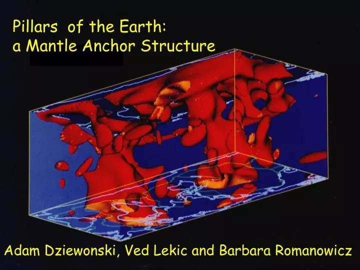
Pillars of the Earth: a Mantle Anchor Structure Adam Dziewonski, VedLekic and Barbara Romanowicz
Two main points: • A very large structure at the bottom of the mantle imposes a permanent imprint on the tectonics at the surface. It determines the band in which subduction can occur and regions of high hot-spot activity. • The characteristics of the spectrum of heterogeneity as a function of depth indicates the presence of five different regions: three in in the upper mantle and two in the lower mantle.
Data and Model The dominant degree-2 signal is clearly visible in the data; the model at 2800 km depth looks very much like travel time anomalies of S-waves that bottom in the lowermost mantle.
Resonance-like power spectrum Left:power spectra of S362ANI, SAW24B16 at 2800 km and the integrated mass anomaly of model L-B&R. Right: cumulative power spectra of the models.
The nearly-indistinguishable degree 2 structures at 2800 km depth of three global tomographic S-velocity models: (a) S362ANI; (b) SAW24B16; (c) S20RTS. Pink circles indicate paleo-pole locations from the true polar wander reconstructions of Besse and Courtillot, 2002.
Slabs at depth 72 km 362 km 652 km 942 km 1377 km 2102 km From Lithgow-Bertelloni and Richards, 1998 j 2827 km
Slabs and seismic velocities; Degrees 1-12 Power spectra
(left)Power spectra of S362ANI and SAW24B16 at 600 km and the integrated upper mantle mass anomaly of model L-B&R. (right) Correlations between each seismic model and the slab model as a function of angular degree. The dashed lines indicate 95% confidence level.
Comparison of seismic model S362ANI (left column) at 600 km and integrated mass anomaly for slab model L-B&R (right column). The top maps show the velocity model at 600 km and the whole-mantle integrated slab model for degrees 1-18. The bottom row shows degree-2 pattern only (note the changed color scale).
Slow Fast Radial correlation functions (Jordan et al., 1993) of the model S362ANI. Top: Only anomalies slower than average. Bottom: Only faster than average anomalies. Note that the slow anomalies have nearly twice the radial correlation length of the fast anomalies. This indicates that fast anomalies may be more fragmented.
All degrees 2800 km Degree 2 Degrees 2 & 3 Degrees > 3 Figure 7.Comparison of seismic model S362ANI (left column) at 2800 km and integrated mass anomaly for slab model L-B&R (right column). The top maps show the velocity model at 2800 km and the whole-mantle integrated slab model for degrees 1-18. The middle row shows degree-2 pattern only (note the changed colorscale), while the third row shows the combined degree 2 and 3 pattern. The bottom row shows the two models for degrees >3.
Hot spots TZ attenuation Velocity at 2800 km Top: Distribution of hotspots in compilation of Steinberger (2000), colored by log of the associated anomalous mass flux (in 103 kg/s). The map is colored to show the degree 2 pattern of this hotspot distribution weighted by each hotspot's anomalous mass flux. Middle: the degree 2 pattern of attenuation perturbations at 600 km from the QRLW8 model (Gung and Romanowicz, 2004). Bottom: degree 2 pattern of the S-velocity model S362ANI at 2800 km.
Three dimensional view of model S20RTS filtered to degree 6. The red anomalies represent -0.6% iso-surfaces; blue anomalies show +0.6% iso-surfaces. Note that slow anomalies are continuous and form two pillars that reach to the transition zone; fast anomalies are more fragmented, except at the bottom.
Power spectra of three models; Harvard Caltech Berkeley angular degree
Rapid change in the level of heterogeneity Romanowicz (2009)